


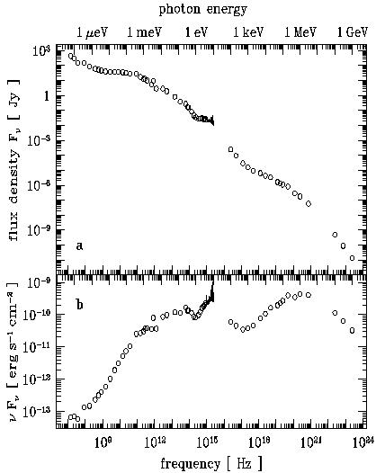
3.5 The Overall continuum spectral energy distribution
Having studied the emission components separately we can now put all
these elements together. To do so we present in
Fig. 8 the average spectrum obtained by
projecting all the data of Fig. 1 onto
the frequency axis.
Figure 8 also gives the same data but in the
form of  .
f versus
. It is striking that the flux
per logarithmic interval is nearly constant over more than ten decades
of frequency, another way of expressing that to the first order the
emission is proportional to
-1. In the second order, it is
striking to see two maxima in the
.
f versus
distribution at roughly the same level, one in the far ultraviolet and
the other at about 1 MeV.
.
f versus
. It is striking that the flux
per logarithmic interval is nearly constant over more than ten decades
of frequency, another way of expressing that to the first order the
emission is proportional to
-1. In the second order, it is
striking to see two maxima in the
.
f versus
distribution at roughly the same level, one in the far ultraviolet and
the other at about 1 MeV.
|
Figure 8. Overall average spectrum of 3C 273
(first panel). This corresponds to a projection onto the frequency axis
of all data in figure 1. The bottom panel shows the same data as above
but represented as |
Integrating the spectrum one can deduce the total flux in the average
spectrum and the bolometric luminosity of 3C 273. One finds a total
flux of 1.9 . 10-9 ergs s-1
cm-2 and assuming
isotropic emission, H0 = 50 km/(s Mpc),
 = 1 and q0 =
0.5 one finds a luminosity of 2.2 . 1047 ergs
s-1.
(Türler et al in preparation).
= 1 and q0 =
0.5 one finds a luminosity of 2.2 . 1047 ergs
s-1.
(Türler et al in preparation).