5.2. General Techniques

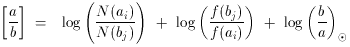
The abundance analysis for absorption lines is, in principle, much simpler than for the emission lines because the absorption yields direct estimates of the ionic column densities. One only has to apply an ionization correction to convert the column density ratios into relative abundances. The logarithmic abundance ratio of any two elements a and b is related to their column densities by,

(1)

where (b / a) is the solar abundance ratio, and N and f are respectively the column densities and ionization fractions of elements a and b in ion states i and j. If the gas is in photoionization equilibrium and optically thin at all far-UV continuum wavelengths, the correction factors, f (b_j) / f (a_i), depend only on the shape of the ionizing spectrum and the ionization parameter U (defined as the dimensionless ratio of the gas to hydrogen-ionizing photon densities at the illuminated face of the cloud).

Figure 6. Ionization fractions in optically thin clouds photoionized at different U by a power-law spectrum with index = -1.5. The HI fraction appears across the top. The curves for the metal ions Mi are labeled at their peaks whenever possible. The notation here is SiII = Si+2, etc.

Figure 6 shows theoretical ionization fractions, f(M_i), for various metals, M, in ion stage, i, as a function of the ionization parameter, U, in optically thin photoionized clouds (from HF99). The HI fraction, f(HI), is shown across the top of the figure. The calculations were performed using CLOUDY (version 90.04, Ferland et al. 1998) with a power-law ionizing spectrum with index = -1.5, where f . Note that the results in Figure 6 are not sensitive to the specific densities or abundances used in the calculations (within reasonable limits, see Hamann 1997). Ideally, we would constrain the ionization state (i.e. U) in Figure 6 by comparing the column densities in different ionization stages of the same element. We can also constrain the ionization by comparing ions of different metals with some reasonable assumption about their relative abundance. With U thus constrained, Figure 6 provides the correction factors needed to derive abundance ratios from Eqn. 1. Repeating this procedure with calculations for different ionizing spectral shapes yields estimates of the theoretical uncertainties (Hamann 1997).

If the data provide no useful constraints on U (because too few lines are measured) or multiple constraints imply a range of ionization states (as in the z_a z_e system of UM 675, Hamann et al. 1995b), we can still derive conservatively low values of f(HI) / f (M_i) and thus [M/H] by assuming each metal line forms where that ion is most abundant (i.e. at the peak of its f (M_i) curve in Figure 6). We can also place firm lower limits on the [M/H] ratios by adopting the minimum correction factor for each M_i. (Every f(HI) / f (M_i) ratio has a well-defined minimum at U values near the peak in the f(M_i) curve.) Hamann (1997) presented numerous plots of the minimum and conservatively small ionization corrections for a wide range of ionizing spectral shapes. Note that the correction factors for some important metal-to-metal ion ratios, such as FeII / MgII and PV / CIV, also have well-defined minima that are useful for abundance constraints (see also HF99 and Hamann et al. 1999).