


Optical surveys over the magnitude range 17  mB
22 are
effective in the sense that to some specified flux
limit the majority of quasars are identified. Evidence supporting this
conclusion comes from the similarity of quasar rest-frame
optical-ultraviolet spectra selected at radio, X-ray and
optical wavelengths (e.g.,
Steidel and Sargent
1991). Surveys based on
the lack of proper motion and the presence of long-term photometric
variability produce surface densities comparable to those from
color-based or slitless spectroscopic techniques, and again, the
spectroscopic properties of the quasars so located are not unusual.
The overall form and normalization of the source counts at the level of
~ 20% are established, but a detailed picture of the quasar
population and its evolution requires a quantitative understanding of the
effectiveness of surveys.
mB
22 are
effective in the sense that to some specified flux
limit the majority of quasars are identified. Evidence supporting this
conclusion comes from the similarity of quasar rest-frame
optical-ultraviolet spectra selected at radio, X-ray and
optical wavelengths (e.g.,
Steidel and Sargent
1991). Surveys based on
the lack of proper motion and the presence of long-term photometric
variability produce surface densities comparable to those from
color-based or slitless spectroscopic techniques, and again, the
spectroscopic properties of the quasars so located are not unusual.
The overall form and normalization of the source counts at the level of
~ 20% are established, but a detailed picture of the quasar
population and its evolution requires a quantitative understanding of the
effectiveness of surveys.
5.1 Completeness
Surveys of the quasar population can be thought of as attempting to compile a census within a comoving volume at a given redshift, z. Each quasar within a comoving volume element can be described by its luminosity at some specified rest-frame wavelength, together with the form of its SED. The term SED is meant in the most general sense, involving specification of the energy output over many decades of frequency, at a resolution sufficient (in the optical and ultraviolet regimes at least) to describe the properties of individual emission lines. The form of the SED together with the reference luminosity (or equivalently an absolute magnitude), which provides the normalization, allow a bolometric luminosity to be derived. Each quasar may be thought of as lying within a three-dimensional space, with axes: absolute magnitude, SED and redshift, or (M, SED, z). Ideally one would like a census of all quasars, brighter than some faint bolometric luminosity, for all redshifts, and such a sample would indeed be ``complete''. However, compilation of such a sample is not possible, and there is no prospect of its becoming possible (for an earlier discussion on this point, see Weedman 1986).
From much of the literature one might conclude that striving for the ``complete quasar sample'' is comparable to King Arthur's quest for the Holy Grail. In the modern quest, a technique for selection is applied, a sample defined, compared with extant samples, and usually claimed to be superior to other work. Papers describing optical quasar surveys, including those on which most of our knowledge of quasar evolution is based, and at least one in which we have both participated, as a rule contain an argument that runs: ``The surface density of quasars found in our survey is as large as in published work, and most previously known quasars in the area were recovered independently, therefore our survey is highly complete.'' Common practice is then to apply a small correction, of order 10%, to the surface or space densities derived and to proceed with the analysis, equivalent to assuming P (M, z, SED) = 0.9 for all SEDs, and some range of M and z. Sometimes different selection techniques are applied to ensure the survey is even more ``complete.''
Given the uncontroversial view with which this section begins, the principle of which applies equally to compiling a census of galaxies or binary stars, it is surprising that surveyists appear so concerned with attaining the ``complete survey of quasars''. In part, the explanation lies in the use of the term complete. Frequently, ``complete'' is used to imply that a specified area of sky has been searched in a consistent and well-defined manner. A more appropriate term is ``well-defined.'' Thus, an ultraviolet-excess survey may be undertaken with precisely specified magnitude and U - B color limits; the survey is well-defined, but in no sense complete. When used in this context we would argue the term complete is something of a misnomer, although its use is extensive.
The ability to constrain theoretical models depends on a survey's being sensitive to a significant dynamic range in the intrinsic properties of quasars. However, surveys are undertaken using the observed properties and the effective utilization of a survey involves two very different steps. The first is the calculation of the effectiveness in terms of the observed properties, e.g., what fraction of quasars with colors B - R = 0.6 are included as a function of R magnitude; the second is the mapping between the observed properties and the intrinsic properties of the quasars, e.g., what constraints on the absolute magnitude and SED of a quasar can be obtained given the redshift, R magnitude and B - R color.
The discussion of ``completeness'' in practically all papers
deals with the first of these two stages. The stated goal is to obtain
a complete sample defined in terms of observed properties. An
implication frequently associated with this approach is that such a
``complete'' survey will result in the definitive understanding of the
quasar population, and furthermore, that if a survey is not complete
then it is fundamentally limited in application. Both contentions are
fallacious. If, for example, some quasars are dust-enshrouded and emit
predominantly at far infrared wavelengths, or, if quasars at z > 3 are
obscured by dust in intervening galaxies, then the attenuation of flux
at ultraviolet and optical wavelengths would have the effect
of removing the objects from any attainable flux-limited sample in
these bands. This is not an extreme or unrealistic example;
if quasars have an intrinsic spread in the line-of-sight extinction
of only  E (B - V)
= 1 mag, the observed spread in B magnitudes for z
~ 2 quasars will be B ~
10 mag! Neutral hydrogen in
the postulated obscuring torus, or intervening galaxy disc, would
produce similar effects in the soft X-ray regime.
This example illustrates that increased dynamic range (in whatever the
observed property) potentially yields more interesting constraints than
``completeness'' within some much narrower range of the observed property.
E (B - V)
= 1 mag, the observed spread in B magnitudes for z
~ 2 quasars will be B ~
10 mag! Neutral hydrogen in
the postulated obscuring torus, or intervening galaxy disc, would
produce similar effects in the soft X-ray regime.
This example illustrates that increased dynamic range (in whatever the
observed property) potentially yields more interesting constraints than
``completeness'' within some much narrower range of the observed property.
The concept that 100% effectiveness is a prerequisite for success is also based on a false premise. The number of quasars detected is proportional to Pdetect x Nquasar, where Pdetect is the probability of detection and Nquasar is the number of quasars falling within the survey. To derive constraints from the observations the product must be significantly non-zero and Pdetect precisely known. For some applications, such as the clustering-related illustration in Section 4.2, it is sufficient that Pdetect is constant, its specific value need not even be known. As discussed in Section 4.1, it is often the case that one of a survey's goals is to set limits on the surface density of undetected hypothetical objects of a certain type (e.g., radio-quiet BL Lac objects). If no such objects are found, then Pdetect x Npredicted, where Npredicted is the number of objects predicted by a model to lie within the survey, must be significantly non-zero in order to critically test the model. Pdetect must be known, but need not be equal to unity.
Selection independent of SED has been proposed to obtain a ``complete'' sample, with the absence of proper motion sometimes cited as such a technique - the rationale of the method being that essentially all Galactic stars will show a detectable proper motion, and spectroscopy of the small fraction of objects with zero proper motion should provide a census of all quasars whose broad-band magnitudes place them within the survey limits. A survey based on proper motion is a prudent check on the effectiveness of other optically-based techniques (Majewski et al. 1991, 1993), however, the flux range over which proper motions can be measured is small relative to the extent of the luminosity function at a given redshift (Section 2.1). The inherent bias which results in quasars with certain SEDs and redshifts being more likely to be included in a particular broadband flux-limited sample applies, so the technique is significantly limited by the dispersion in quasar SEDs.
Once the probability of detection is known as a function of the observed properties, the next step is to perform the mapping from observed to intrinsic properties. Derivation of the luminosity function at some redshift requires flux in the observed-frame to be related to a bolometric luminosity, or at least to a luminosity at a specified rest-frame wavelength. Since quasars are selected using observed properties, no survey is unbiased with respect to the intrinsic properties of quasars. For example, a flux-limited survey performed at a particular waveband will include relatively more quasars at certain redshifts with strong emission lines than objects with weak emission lines. Quasar surveys are always biased in this sense and the ability to derive the intrinsic distribution of properties depends on being able to quantify the experiment so that the unavoidable bias may be corrected. Determining the selection function provides the means to undertake this task. Since a quasar's contribution to the space density, or to a census of SEDs, is proportional to 1 / P, the intrinsic fraction with small values of P (M, z, SED) can be large. Quasars with such unusual SEDs may be important for constraining models involving orientation-dependent effects, or extreme conditions in the continuum- and broad-line-emitting regions; calculation of the selection function ensures the contribution of such objects is correctly incorporated.
Until recently the transformation between observed and intrinsic
properties has been carried out assuming that all quasars have
identical SEDs, and that the universal SED may be represented by a
power-law relation in frequency, with (in the optical) the addition of
``mean'' emission-line fluxes for the strongest features such as C IV
 1549 and Lyman-
 . The procedure is identical
at other wavelengths, but because of the simpler form of the SEDs and the
lower-resolution of the observations, the mapping of the observed flux
to intrinsic luminosity is performed using power-law approximations to
the SEDs alone. The concept of allowing for different SEDs was
incorporated into analyses of radio-selected samples through the
treatment of ``flat-spectrum'' and ``steep-spectrum'' populations.
. The procedure is identical
at other wavelengths, but because of the simpler form of the SEDs and the
lower-resolution of the observations, the mapping of the observed flux
to intrinsic luminosity is performed using power-law approximations to
the SEDs alone. The concept of allowing for different SEDs was
incorporated into analyses of radio-selected samples through the
treatment of ``flat-spectrum'' and ``steep-spectrum'' populations.
5.2 Survey Quantification
To derive quantitative results it is necessary to actually determine P (M, z, SED). Given the lack of significant differences in the spectroscopic properties of quasars selected using different techniques (e.g., Baldwin, Wampler and Gaskell 1989, Steidel and Sargent 1991) it is likely that we have a fair estimate of the range of SEDs present in the population (with the exception of extreme objects such as quasars whose SEDs are significantly reddened by dust). What remains unknown is the intrinsic proportions of objects as a function of SED. Detection probabilities are required for the full ranges of luminosity, redshift and SED, at a resolution such that the probabilities do not change significantly from one redshift interval to another, or between adjacent SED ``types.'' Since the relative proportions of SED types among the quasar population are unknown, the true distribution of types has to be calculated simultaneously with the intrinsic distributions in redshift and absolute magnitude.
There are two reasons that the calculation of selection functions has not been attempted more frequently. The first is the lack of data in digital form; much important work involved visual inspection of survey material, e.g., the Canada-France-Hawaii Telescope grens surveys of Crampton and collaborators (Crampton, Cowley, and Hartwick 1989). Human-based selection cannot be precisely specified and hence it is not possible to determine the array of probabilities P (M, z, SED). The second reason is the complexity of the calculation. The time between the compilation of the observational data, i.e., obtaining the follow-up spectroscopy of the candidate objects, and the completion of the analyses by Schmidt et al. (1994) and Warren, Hewett and Osmer (1994) attests to the degree of difficulty. In most cases the calculation of the array of probabilities P (M, z, SED) is more onerous than the completion of the candidate identification and spectroscopy.
Warren et al. (1994) derive P (M, z, SED) by introducing artificial quasars into the observational data set, and this approach is essential for many optical surveys. The principle is the same as that employed in assessing the incompleteness of photometric catalogs in globular clusters (e.g., Stetson 1987) although there are more factors that must be taken into account when considering the quasar experiment. The multicolor work provides a good example of the calculation of P (M, z, SED) and a brief description is given here.
The procedure commences with the generation of a synthetic quasar spectrum as it would appear above the atmosphere. The spectrum is characterized by a power-law continuum, an accretion disc component, and an emission line component. Colors are calculated by allowing for the effects of atmospheric transmission and then convolving the spectrum with the known response functions of the emulsion plus filter combinations. Colors in the survey system for an object with specified M, z and SED can thus be generated readily. However, additional factors influence the observed colors and these must be incorporated. The first is the error in the magnitude determination for each color band. The second, is the influence of intervening absorbers on the quasar spectrum; the effect on a quasar spectrum depends on the number and properties of the clouds between us and the quasar, so the synthetic quasar will appear different along each line of sight. Finally, the photographic plates used were not all taken contemporaneously and the intrinsic variability of the quasar will introduce an additional scatter into the observed colors.
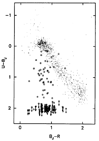
The quantification process requires a precise specification of the magnitude errors and a detailed models for the intervening absorbers (and their effects on the quasar spectrum), and the variability behavior as a function of time. With these in place the selection function calculation proceeds by considering each quasar, of specified M, z, SED, and taking 100 realizations of its appearance within the data set. In each realization the effects of magnitude errors, photometric variability and intervening absorbers are incorporated by drawing randomly from their statistical distributions. Figure 2 illustrates the results of the procedure for a simulation with properties very similar to one of the quasars identified in the survey. The exact determination of the probability of selection involves adding each realization in turn to the actual data set and applying the selection algorithm employed to identify the candidates. In Figure 2, different symbols are used to indicate which realizations of the particular object would have been included in the candidate list. The final result is the number of realizations that would have been included, divided by 100. Increased precision is possible by increasing the number of realizations.
|
Figure 2. U - BJ vs. BJ -
R projection of the six-dimensional
color-space used to select quasars by Warren et al. (1994). The
colors of 1000 stellar objects, of the total of 29,815, in one of
the survey fields are shown as small dots. The distribution is marked
by the well-defined main-sequence of stars extending from A-stars
with colors U - BJ = BJ - R ~ 0 to
M-stars at lower right. A cloud of white-dwarfs and low-redshift quasars
is visible at top left. The location of a z = 3.33 quasar with
colors BJ - R = 0.98 and U - BJ =
2.1 is identified by an x and downward arrow; the arrow
indicating that the object was not visible on the U plates, hence
only a lower-limit for the U - BJ color is available.
The circle and square symbols mark the locations of 100
realizations of a synthetic quasar with properties very similar to the
z = 3.33 quasar located in the survey. Arrows again denote lower limits
to the U - BJ color, indicating that in a particular
realization the
U magnitude was fainter than the plate limit. The synthetic quasar
has specified redshift, continuum and emission line properties.
Magnitude errors, variation in the hydrogen absorption along different
lines-of-sight, and a dispersion in the quasar magnitudes arising
from photometric variability all contribute to the spread in the
distribution of the simulations. The large extent in U -
BJ is due
primarily to the variation in hydrogen absorption, with most
lines-of-sight heavily absorbed, producing the group of points at the
bottom of the plot, while clearer lines-of-sight produce more flux in
the U band for a smaller fraction of the simulations. The magnitude
errors are relatively small,  ~ 0.1, and the spread in BJ - R arises mostly from the
effects of quasar photometric variability coupled with the large epoch
difference of the BJ and R plates.
Each realization is introduced into the full data set, including all 29,815
objects in the field, and the algorithm used to identify the candidates
in the survey is applied. Realizations indicated by circles would have
been included in the sample while those marked squares would not have
been high enough up the candidate list for a follow-up spectrum to
have been obtained. Twenty-two of the realizations escape detection,
leading to an estimate of P (M, z, SED) for the object of ~ 0.78.
~ 0.1, and the spread in BJ - R arises mostly from the
effects of quasar photometric variability coupled with the large epoch
difference of the BJ and R plates.
Each realization is introduced into the full data set, including all 29,815
objects in the field, and the algorithm used to identify the candidates
in the survey is applied. Realizations indicated by circles would have
been included in the sample while those marked squares would not have
been high enough up the candidate list for a follow-up spectrum to
have been obtained. Twenty-two of the realizations escape detection,
leading to an estimate of P (M, z, SED) for the object of ~ 0.78.
|
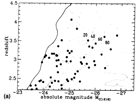
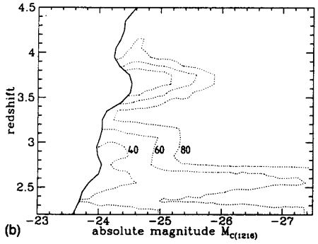
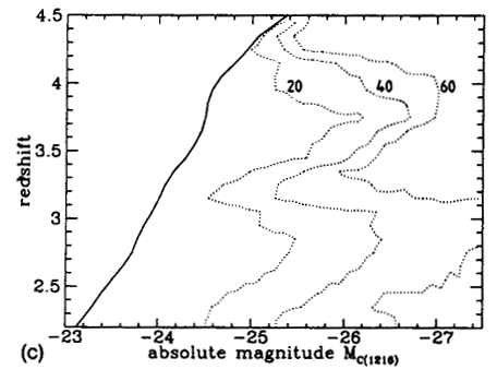
Following the calculation for a full array of SEDs, z and apparent magnitude, contour plots of the effectiveness of the survey can be constructed. Figure 3 shows the results for three different SED types. In the central panel the quasars located in the well-defined sample are shown overlaid on the contours of detection probability. A full description of the parameters defining the procedure can be found in Warren et al. (1994).
|
|
|
| Figure 3. (a) Absolute magnitude vs. redshift distribution of quasars located in the multicolor survey of Warren et al. (1994). The heavy line at left is the absolute magnitude limit at each redshift corresponding to the limiting apparent magnitude, mR = 20 of the survey. The contours show the probability of identifying an object of specified absolute magnitude and redshift. The calculation has been performed for a quasar with typical continuum and emission line properties. Contour levels are labeled with the value of 100 x P (M, z, SED). (b) As in (a), but contours are shown for a quasar with a relatively blue continuum and strong emission lines. Note how the absolute magnitude cutoff at each redshift has shifted compared to (a) because the relation between absolute magnitude and apparent magnitude changes as a function of SED. The more pronounced ``waves'' in the limit occur because the emission lines are stronger. The individual quasars are omitted from the plot for reasons of clarity. (c) As in (b), but contours are shown for a quasar with a red continuum and weak emission lines. Again, note the difference in the form of the cutoff resulting from the survey apparent magnitude limit and the significant difference in the probabilities of detection as a function of SED. Full details of the parameters describing the synthetic quasars may be found in Warren et al. (1994). |
5.3 Analysis and Models
Ideally, one classifies where each detected quasar lies within the M, z, SED space, and divides the number in that region by the associated probability of detection to infer the true number of such objects that would be found, were the detection probabilities unity. In practice the range of absolute magnitude, redshift and SEDs of interest and the non-uniform distribution of quasars as a function of these variables means that the signal-to-noise ratio is too low. Instead, a model for the distribution of quasars in the M, z, SED space can be taken, convolved with the associated probabilities of detection, and compared with the observed distribution. Maximum-likelihood techniques for deriving model parameter values were introduced by Marshall (1985), and statistics such as the two-dimensional Kolmogorov-Smirnov test (Peacock 1983) to quantify the goodness of fit, enable the procedure to be accomplished relatively easily. The true proportions of quasars as a function of SED must be calculated at the same time that the luminosity function and evolution parameters are being derived. An important advantage of this approach is that the data, the quasar fluxes, redshifts and SEDs, can be used directly to constrain the model. The model is manipulated to take account of accessible volumes, photometric errors and the detection probabilities, and to provide predictions of the distribution of observed fluxes, redshifts and SEDs. This manipulation can be achieved to an arbitrary precision and the simplicity of this approach contrasts markedly with the problems involved in attempting to transform the (noisy) data into the model plane.
The disadvantage of this approach, is the parametric nature of the
procedure, which requires specifying the model a priori rather
than allowing the data to determine directly, for example, the form of
the luminosity function and its evolution with redshift. The object is
to establish whether the model is consistent with the data, not to
establish that the model is correct. In the 1980s a variety of
apparently contradictory conclusions were published concerning the form
and evolution of the luminosity function at redshifts z  3.
Much of the apparent disagreement can be ascribed to the restricted
nature of the analysis. Often, a particular model for the evolution was
shown to be consistent with the survey results. What was not
established was the full range of models consistent with the
data. There are few inconsistencies between the results
(Warren and Hewett
1992; Section 7), but the surveys do
not offer very strong, and hence
interesting, constraints. i.e., a large range of models is consistent
with the very limited data. More recently, both the design of surveys
and their analysis has become better suited to the scientific goals and
it is now common to explore a much wider range of model
parametrizations.
3.
Much of the apparent disagreement can be ascribed to the restricted
nature of the analysis. Often, a particular model for the evolution was
shown to be consistent with the survey results. What was not
established was the full range of models consistent with the
data. There are few inconsistencies between the results
(Warren and Hewett
1992; Section 7), but the surveys do
not offer very strong, and hence
interesting, constraints. i.e., a large range of models is consistent
with the very limited data. More recently, both the design of surveys
and their analysis has become better suited to the scientific goals and
it is now common to explore a much wider range of model
parametrizations.