

Since most of you who are here today are experts in the field of spectral classification, all that I shall try to do is to share some of my many mistakes with you. Of course, I do not pretend to know anything about stars earlier than G0, so let us talk only about the later types.
First, I want to correct a misunderstanding which I hope is not shared by many. It has been said that when classification is carried out by visual inspection of spectrograms the process is purely subjective, and that the classifier is free to make arbitrary changes in the scheme of types assigned to the stars. This is untrue! It is subjective only in the sense that the ability of the human eye to match complex patterns is used, but the network of patterns defining the system is the same whether the comparison is made visually or by summing measured intensity ratios, or by deriving an electronic pattern recognition index. If I or anyone else made arbitrary changes in a system, that system would soon cease to be useful.
As is emphasized so strongly by Morgan (1984) in this volume, one is justified in modifying the system itself usually for one reason only: to make the types describe the actual spectra more accurately.
Of course, the criteria must be kept flexible in order that they can be adapted to different dispersions and instrumental response curves, but the scheme of classification is essentially defined in terms of the set of reference stars. One thing that I have learned by bitter experience is that the cool stars, and practically all supergiants, cannot be trusted to remain constant in their spectral features. That compels us to use as many standards as possible, and to have enough observations of each to give us some confidence that we are defining a reliable average type. This is an important difference as compared to the greater constancy of many of the standard stars of earlier type.
When we come to the second stage of classification, the calibration of the types against physical variables, a practical problem often arises. For example, what should we do if someone improves the scale of effective temperatures of the stars, and we find that when we plot the types against some known function of temperature an irregular curve results? We should not change the spectral types to obtain a smoother relationship, but we can do just what we did when we inherited the letter types from the old Henry Draper system; we do not treat all the possible decimal subdivisions of the types as full subtypes, but we make some adjustment in their spacing when we plot our calibration curves.
It is only the full subdivisions that are plotted at equal intervals, and the practice that I and most others are following now for types between G0 and M8 is shown in the first column of table 1. Within type G there have been no recent changes, and the only full subtypes recognized are G0, G2, G5 and G8. The other possible subdivisions are utilized only for interpolation whenever we think that we can classify accurately enough to justify their use. Thus when we call a star G3 we mean only that it is closer to G2 than to G5.
| G0: 30 | K1: 35 | M0 40 | M4: 45 |
| G2: 31 | K2: 36 | M1: 41 | M6: 46 |
| G5: 32 | K3: 37 | M2: 42 | M7: 47 |
| G8: 33 | K4: 38 | M3: 43 | M8: 48 |
| K0: 34 | K5: 39 | M4: 44 | |
In a similar way, it has long been recognized that K5 and M0 are only about one subtype apart. We can easily distinguish half-subtypes here, and assign K7 to many stars, but it happens that just at this point in the giant branch, when the strongest TiO bands begin to become visible, our criteria are sensitive to very small differences in temperature, which present methods of measuring Tef cannot well distinguish. Hence, if K7 is plotted as a full subtype the change of slope of any calibration curve of type versus Tef is exaggerated.
These points that I have been making must seem very obvious to most experienced classifiers, but are frequently misunderstood by others who use spectral types. Users are also sometimes puzzled by our occasional changes in the spectral types of even the brighter stars. Of course, it might be more convenient if spectral types were engraved in granite, but they are measured quantities and as such must be refined as our observations improve. Sometimes it is just a matter of obtaining spectrograms of better quality, but for such stars as the most luminous supergiants, the number that were known when the original MK System was set up was very small, and as we fill in the sequence with more stars it sometimes becomes apparent that our sets of standards would become more consistent if slight shifts were made in the types of the ones first classified.
An example of a mistake resulting from a desire to keep things simple was the old system of classifying S-type stars that I proposed in 1954. At that time it seemed reasonable to assume that the passage from type M to type S corresponded to a change in essentially one abundance parameter; the ratio of heavy elements to lighter elements as measured by the band ratio ZrO/TiO. Later the work of Scalo and Ross (1976), Ake (1978, 1979) and others showed that the ratio C/O differed systematically between the two groups of stars, and when Pat Boeshaar and I (1979, 1980) revised the classification of the M-S-SC-C sequence we were obliged to allow for the possible variation of both parameters. There is pretty good evidence that there is not always a one-to-one correspondence between C/O and Zr/Ti, and it may eventually be necessary to specify even more abundance parameters in order to define the subgroups.
Of course, it would be easier to dodge the issue and stick to the original MK System and just give a two-dimensional classification applicable mainly to Population I stars like the Sun in composition. However, I agree with Madame Cayrel that a scheme that just puts a ``p'' (for ``peculiar'') after the type of every star which does not fit is not very helpful to anyone. I believe that we owe, it to the theoreticians to provide types that will suggest what abundances they should vary in constructing realistic models that will account for the observed spectra. The types should serve also to point out the stars that are worth individual analysis.
The Revised MK Classification for the cooler stars is a multi-dimensional system in which abundance indices are added to the temperature types and luminosity classes - but only when certain lines and bands in a spectrum indicate apparent abundance differences as compared to Population I stars of solar composition. I think that this development is consistent with the definition of the MK Process given by Morgan (1984) in this volume.
There are, however, some kinds of stellar spectra that cannot now be fitted into the boxes of even this expanded system. One extreme group is that of the red carbon stars. When the C-classification of them was proposed in 1941 (Keenan and Morgan 1941), we tried to use criteria, such as the D lines and relative band strengths, that might be expected to give a reasonably good temperature sequence. However, the tangle of overlapping bands of C2 and CN, which leaves no real continuum from which intensities of absorption features can be reliably estimated, pretty well obscures the temperature effects, except in the hotter R stars. The sensitivity of the band strengths themselves to abundance effects adds to the confusion. I think that Yamashita (1972, 1975) has done the job of classifying carbon stars on this system as well as anyone could do it, but the criteria available are just not good enough. While those who say that the C types show an anticorrelation with temperature have not made a very good case, I must agree that the correlation is very poor.
Now, what can we do to make a real improvement in the accuracy of spectral types, and in their sensitivity to the fundamental physical variables, not only for such recalcitrant groups but for stars in general? It makes sense to try the obvious courses of action first. These are:
Consider the spectral regions first. Nearly all of the former and present schemes of classification based on photography were fortunate in being practically limited to the blue, yellow, and red regions, where the photospheric light could be observed. This means that the types are at least consistent in referring to the lower atmospheres, where the ionization and excitation temperatures can be correlated with the effective temperatures of the star. To put it in another way, we were led by necessity to work close enough to the star's black-body maximum to observe conditions as far down in the atmosphere as possible.
This is not true of other spectral regions. To oversimplify and belabor the obvious, in the ultraviolet we are observing chromospheres (and in the X-ray region, coronae) and in the infrared, for the brightest supergiants and very cool stars in general, we are observing detached shells of dust.
Of course, it is immensely important to study the spectra of these regions, but we should not expect that any kind of classification that we work out for them will necessarily correlate well with MK types.
This severe limitation does not prevent us from improving our spectral coverage, for we have not made enough use of the yellow and red regions in the past. For M stars, for example, the bands of both the singlet and triplet system of TiO in the orange provide a good opportunity to use ratios of bands arising by absorption from different lower levels in assigning temperature types. The ratios of VO to TiO bands in this region are also useful for types later than M6 (Keenan 1963). Those of us who classify from spectra in the blue region, and many of those who use narrow-band photometric classification in any region, tend to rely too much on the strengths of individual bands. I have the uncomfortable feeling that we have failed to recognize population effects on absolute band strengths in some stars.
A promising development has been the design of new split-beam
spectrographs at both the Mount Wilson and Royal Observatories that
will permit simultaneous records of the blue and red regions to be
obtained at classification dispersions. These should permit better
classification of the banded spectra of cooler stars. As far as
extension of the spectral range is concerned, the only other
possibility that I can suggest now is utilization of the features
between  6850 and 8500 Å that have
usually been submerged under the
telluric bands of O2 and H2O. These include the
several bands in S
stars that have been only partially identified. Observations need to
be made from elevations high enough to be above the terrestrial
absorbing layers, but the difficulty is to obtain sufficient observing
time there to carry out lengthy programs of classification.
6850 and 8500 Å that have
usually been submerged under the
telluric bands of O2 and H2O. These include the
several bands in S
stars that have been only partially identified. Observations need to
be made from elevations high enough to be above the terrestrial
absorbing layers, but the difficulty is to obtain sufficient observing
time there to carry out lengthy programs of classification.
Turning now to the question of resolution, the greatest handicap
that we face in classifying any star cooler than the Sun is the severe
blending that affects almost all the features that are sensitive to
the physical variables that we are trying to separate. If you look in
any atlas of spectral types, you will find the feature at 4077 Å
marked as an ultimate line of Sr II, and used as an important
criterion in estimating luminosity of the stars. Actually, however,
this line is blended with rather strong lines of Y I, La II, Dy II and
Fe I (4078). The iron line is
not sensitive to luminosity, while
abundance of the heavy elements is an important factor in determining
the strength of the other contributors.
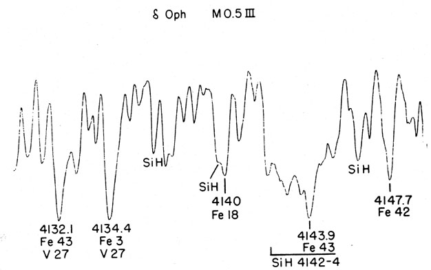
|
Figure 1. SiH in the |
Consider now the strong feature at 4143 Å. We optimistically refer
to it as a line of neutral iron, but in giants from K3 to early M, you
can see in the intensity tracing (figure 1) made
from a Palomar
spectrum (at 9 Å/mm) of the M0.5 giant  Oph, that the iron line is
not very conspicuous at one edge of the compact band due to the SiH
molecule. As
Dorothy Davis (1940)
first showed, the SiH band becomes
conspicuous in giants near K2 and reaches a maximum around M1. Nearly
every feature in this region is somewhat distorted by SiH absorption
in these normal stars. I have suspected 4143 of being unusually
strong in some stars, but from low-dispersion spectrograms alone there
is no way to tell whether this might be an abundance effect in the SiH
bands; the possibility needs to be investigated. This would be a
promising thesis problem.
Oph, that the iron line is
not very conspicuous at one edge of the compact band due to the SiH
molecule. As
Dorothy Davis (1940)
first showed, the SiH band becomes
conspicuous in giants near K2 and reaches a maximum around M1. Nearly
every feature in this region is somewhat distorted by SiH absorption
in these normal stars. I have suspected 4143 of being unusually
strong in some stars, but from low-dispersion spectrograms alone there
is no way to tell whether this might be an abundance effect in the SiH
bands; the possibility needs to be investigated. This would be a
promising thesis problem.
Now let us move over to the 4554 Å line of ionized barium, which
defines a barium star when it is strong enough to stand out clearly at
classification dispersions. Figure 2 [plate 4]
shows a Perkins
low-dispersion classification spectrogram compared to a Palomar coudé
plate, taken several years ago by Olin Wilson and myself. The star is
o Vir, G8 III Ba 1. The barium index is just strong enough to allow us
to call it a true barium star, though not a strong one. The 4554 Å
line is only slightly stronger than the neighboring lines of Ti and
Fe. If it were any weaker the classification spectrogram would show
only a slight enhancement, and the object would be called a marginal
barium star (with fractional barium index). Objective-prism
spectrograms generally have lower resolution than our 75 Å/mm plate,
so you can see why only the stronger barium stars can be picked up
with certainty on objective-prism surveys.
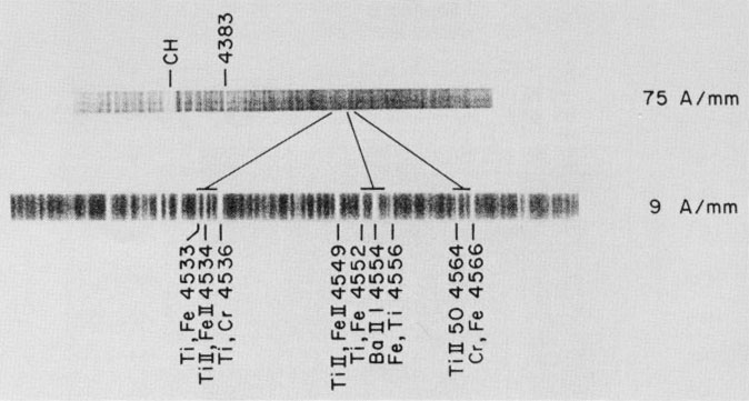
|
Figure 2. |
I shall give just one more example of the problems caused by
blending, which shows that even in the fourth edition of The Bright
Star Catalogue there are stars that have not been well classified or
analyzed. Recently Bidelman asked me about HR 965, which is listed as
a spectroscopic binary with a composite spectrum, G3 IIp + F0: V, but
which he thought might have slightly strengthened Ba 4554. The star
had been recognized as a spectroscopic binary in the early work done
at Victoria
(Plaskett 1921)
at about 30 Å/mm.
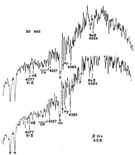
|
Figure 3. Figure 3. Comparison of HR 965
with a bright giant ( |
Fortunately my former observing assistant, Wereb, had obtained good
classification spectrograms with the Perkins Telescope at the Lowell
Observatory in Flagstaff, and a slightly smoothed intensity tracing is
reproduced in the lower part of figure 3. It is
easily seen that it is
a G-type CH star with slightly weak metal lines. The enhancement of
the G-band had been noticed earlier
(Keenan and Keller
1953).
The strong absorption by CH is shown not only by the G-band, but also by
the enhancement of the 4325
line, which is marked by the arrow in
figure 3. The strongest atomic contributor to
this blend is Fe (42)
at 4325.8 Å, but the very compact 2,2 band of the CH system extends
from 4323 to
4325 Å, and at low
resolution the entire complex
appears merely as a slightly widened line. At resolutions better than
1 Å the depth of the CH absorption can be measured independently of
the iron line.
To get a better idea of what CH absorption can do to the spectrum,
let us look at one of the carbon CH stars
(figure 4), where the CH
features are much stronger. In the diagram it is easy to see the
absorption (P-branches) which starts redward from H and nearly blots
out the normally strong 4383
iron line. The K-branches extend
shortward from the G-band itself and reduce the great 4227 line of
calcium to a weak feature. Of course, these extreme effects are not
seen in a star like HR 965, but the CH absorption probably contributes
to the line weakening throughout the blue region. This makes it
difficult to use the usual luminosity criteria, but the general
agreement with the spectrum of the bright giant
and nearly blots
out the normally strong 4383
iron line. The K-branches extend
shortward from the G-band itself and reduce the great 4227 line of
calcium to a weak feature. Of course, these extreme effects are not
seen in a star like HR 965, but the CH absorption probably contributes
to the line weakening throughout the blue region. This makes it
difficult to use the usual luminosity criteria, but the general
agreement with the spectrum of the bright giant  Crv (G5 II) suggests
that HR 965 is more luminous than the so-called subgiant CH stars
studied by Bond. Incidentally, since the six G-type CH stars analyzed
by Luck and Bond (1982)
were found by them to have an average C/O =
1.2, most of these stars would show calcium bands and be called carbon
stars if they were cooler.
Crv (G5 II) suggests
that HR 965 is more luminous than the so-called subgiant CH stars
studied by Bond. Incidentally, since the six G-type CH stars analyzed
by Luck and Bond (1982)
were found by them to have an average C/O =
1.2, most of these stars would show calcium bands and be called carbon
stars if they were cooler.
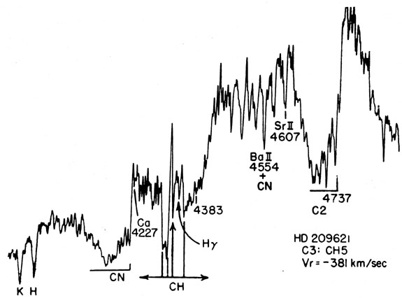
|
Figure 4. The high-velocity carbon CH star HD 209621. CH absorption is shown extended both longward and shortward from the G-band. |
The best type that I can give to HR 965 is G5 II: CH 1 Fe - 1 Ba 0.4, but for the reasons that we have seen it is rather uncertain. If the luminosity class is accepted, the large proper motion implies a space velocity of about 179 km/s. Thus the star is a least a moderate Population II object, which would be expected to show some weakening of the metal lines.
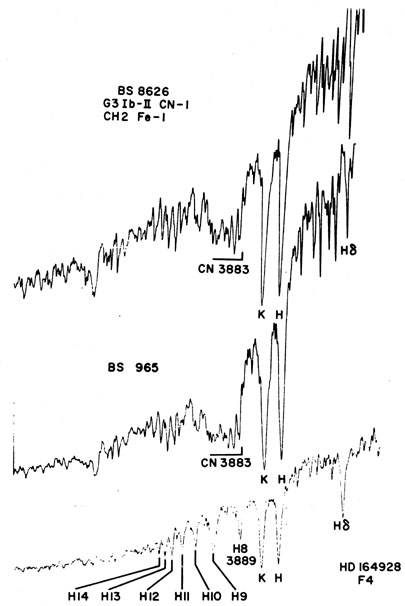
Thus we have two sources of line weakening in HR 965, and when they are taken into account I see nothing to suggest a composite spectrum due to the presence of the companion. If we look farther to the violet (figure 5), and compare HR 965 with an F4 star as well as with the probable supergiant CH star HR 8626, there seems to be no evidence of contamination by an F-type spectrum. I should guess that the companion might be an F8 dwarf, which would be at least 4 magnitudes fainter than the primary even at 3700 Å. Obviously, the star is a prime target for detailed analysis.
|
Figure 5. HR 965 shortward of H and K. In
HD 164928 the apparent
weakness of H, K, and H |
I have gone into this much detail about one star in order to remind you not so much of what can be done at the usual classification dispersions, but of the severe limitations imposed by blending - limitations that can only be overcome by moving to higher resolutions.
If I could start my life over again, I would undertake spectral classification at a resolution no worse than 1 Å, and as much better than that as possible.
In the past, any suggestion that classification should be done at high dispersions has been ridiculed for two good reasons.
First, the exposures for conventional coude spectrograms would be too long. This difficulty, however, is being rapidly overcome with modern detectors. I understand, for example, that with the Arizona-Smithsonian multiple-mirror telescope, stars of the 18th magnitude are already being reached at a resolution of about 1 Å, with reasonable integration times.
The second, and more cogent, objection is that if you can record a spectrum at high resolution, you might as well have your computer carry out an atmospheric analysis and end up with actual abundances. The answer to that argument is twofold. First, the luminosities and temperatures of cool giants and supergiants are still not as well established as we would like for even the most normal stars. Second, as Dr. Mihalas emphasizes in this volume, the atmospheric models still need much improvement, especially at the low temperatures at which molecular formation becomes important. I am confident that the model-makers will gradually make better and better ones, but it should not be necessary to change our catalogues whenever the models for some group are refined.
But if we are going to move to higher resolutions, automatic methods of classification will be even more essential in carrying out surveys of considerable numbers of stars than they are in doing low-dispersion classification. Among the hundreds or thousands of lines in the spectral region that can be registered, the task of finding and comparing the many faint criteria that are useful is just too time-consuming by any of the older methods.
I leave it to the experts in automation to decide on the best techniques, but think that there is one condition that should be met by whatever method is used. It should always be possible to recall or produce quickly the complete spectrum of any star for examination. For example, if one is undertaking pattern recognition by correlation coefficients, the only indication of a peculiar spectrum may be given by the absence of a good correlation with any one of the grid of standards. That will not tell you whether all the lines in the star being classified are wide (or double), or whether just one or a few features have abnormal intensity. To tell what is going on, one must be able to examine the actual spectrum.
Also, if your method involves sampling only narrow spectral regions selected to contain especially sensitive criteria, an outstanding peculiarity outside that region might go completely undetected. That is a problem which is just as acute for people doing photometric classification in narrow or medium bands.
But the existence of these dangers will just make high-resolution
classification of the future all the more exciting. Even for some of
the most ordinary stars the improvement in classification will be
marked; for example, I think everyone will be surprised by the
accuracy with which luminosities will be estimated for G and K
giants. With a resolution of about 1 Å, or slightly better, one can
make use of the positive luminosity effect in the slightly forbidden,
zero-volt, intersystem lines of iron, such as 4258 Å. When a
resolution of about 0.2 Å is available, the ionized lines of Fe and Ti
can be compared with neutral lines of the same elements. In both cases
we do not need to worry about the intrusion of abundance effects.
I envy the young spectroscopists who are working, or will work, in this field and will solve its problems.
 -2II system is at