6. THE TENSOR HARMONIC EXPANSION

The last two sections have pulled a fast one. We began by discussing polarization as a two component tensor quantity, but then started discussing the production of polarization as if only its amplitude were relevant. A more complete formalism for describing the polarization field has been worked out and will be presented in this section (see Kamionkowski, Kosowsky, and Stebbins (1997) for a more extensive discussion). An equivalent formalism employing spin-weighted spherical harmonics has been used extensively by Zaldarriaga and Seljak (1997). Note that the normalizations employed by Seljak and Zaldarriaga are slightly different than those adopted here and by Kamionkowski, Kosowsky, and Stebbins (1997).

The microwave background temperature pattern on the sky T() is conventionally expanded in a complete set of orthonormal basis functions, the spherical harmonics:

(25)

where

(26)

are the temperature multipole coefficients and T₀ is the mean CMB temperature. Similarly, we can expand the polarization tensor for linear polarization,

(27)

(compare with Eq. 8; the extra factors are convenient because the usual spherical coordinate basis is orthogonal but not orthonormal) in terms of tensor spherical harmonics, a complete set of orthonormal basis functions for symmetric trace-free 2 × 2 tensors on the sky,

(28)

where the expansion coefficients are given by

	(29)
	(30)

which follow from the orthonormality properties

	(31)
	(32)

These tensor spherical harmonics have been used primarily in the literature of gravitational radiation, where the metric perturbation can be expanded in these tensors. Explicit forms can be derived via various algebraic and group theoretic methods; see Thorne (1980) for a complete discussion. A particularly elegant and useful derivation of the tensor spherical harmonics (along with the vector spherical harmonics as well) is provided by differential geometry (Stebbins, 1996). Given a scalar function on a manifold, the only related vector quantity at a given point of the manifold is the covariant derivative of the scalar function. The tensor basis functions can be derived by taking the scalar basis functions Y_lm and applying to them two covariant derivative operators on the manifold of the two-sphere (the sky):

(33)

and

(34)

where _ab is the completely antisymmetric tensor, the ``:'' denotes covariant differentiation on the 2-sphere, and

(35)

is a normalization factor. Note that the somewhat more familiar vector spherical harmonics used to describe electromagnetic multipole radiation can likewise be derived as a single covariant derivative of the scalar spherical harmonics.

While the formalism of differential geometry may look imposing at first glance, the expansion of the polarization field has been cast into exactly the same form as for the familiar temperature case, with only the extra complication of evaluating covariant derivatives. Explicit forms for the tensor harmonics are given in Kamionkowski, Kosowsky, and Stebbins (1997). Note that the underlying manifold, the two-sphere, is the simplest non-trivial manifold, with a constant Ricci curvature R = 2, so the differential geometry is easy. One particularly useful property for doing calculations is that the covariant derivatives are subject to integration by parts:

(36)

with no surface term if the integral is over the entire sky. Also, the scalar spherical harmonics are eigenvalues of the Laplacian operator:

(37)

The existence of two sets of basis functions, labeled here by ``G'' and ``C'', is due to the fact that the symmetric traceless 2 × 2 tensor describing linear polarization is specified by two independent parameters. In two dimensions, any symmetric traceless tensor can be uniquely decomposed into a part of the form A_{: ab} - (1/2)g_abA_{: c}^c and another part of the form B_{: ac} ^c_b + B_{: bc} ^c_a where A and B are two scalar functions. This decomposition is quite similar to the decomposition of a vector field into a part which is the gradient of a scalar field and a part which is the curl of a vector field; hence we use the notation G for ``gradient'' and C for ``curl''. In fact, this correspondence is more than just cosmetic: if a linear polarization field is visualized in the usual way with headless ``vectors'' representing the amplitude and orientation of the polarization, then the G harmonics describe the portion of the polarization field which has no handedness associated with it, while the C harmonics describe the other portion of the field which does have a handedness (just as with the gradient and curl of a vector field).

This geometric interpretation leads to an important physical conclusion. Consider a universe containing only scalar perturbations, and imagine a single Fourier mode of the perturbations. The mode has only one direction associated with it, defined by the Fourier vector k; since the perturbation is scalar, it must be rotationally symmetric around this axis. (If it were not, the gradient of the perturbation would define an independent physical direction, which would violate the assumption of a scalar perturbation.) Such a mode can have no physical handedness associated with it, and as a result, the polarization pattern it induces in the microwave background couples only to the G harmonics. Another way of stating this conclusion is that primordial density perturbations produce no C-type polarization as long as the perturbations evolve linearly. This property is very useful for constraining or measuring other physical effects, several of which are considered below.

Finally, just as temperature fluctuations are commonly characterized by their power spectrum C_l, polarization fluctuations possess analogous power spectra. We now have three sets of multipole moments, a_(lm)^T, a_(lm)^G, and a_(lm)^C, which fully describe the temperature/polarization map of the sky. Statistical isotropy implies that

(38)

where the angle brackets are an average over all realizations of the probability distribution for the cosmological initial conditions. Simple statistical estimators of the various C_l's can be constructed from maps of the microwave background temperature and polarization.

For Gaussian theories, the statistical properties of a temperature/polarization map are specified fully by these six sets of multipole moments. In addition, the scalar spherical harmonics Y_(lm) and the G tensor harmonics Y_(lm)ab^G have parity (- 1)^l, but the C harmonics Y_(lm)ab^C have parity (- 1)^{l + 1}. If the large-scale perturbations in the early universe were invariant under parity inversion, then C_l^TC = C_l^GC = 0. The arguments in the previous paragraph about handedness further imply that for scalar perturbations, C_l^C = 0. A question of substantial theoretical and experimental interest is what kinds of physics produce measurable nonzero C_l^C, C_l^TC, and C_l^GC. This question is addressed in the following section.

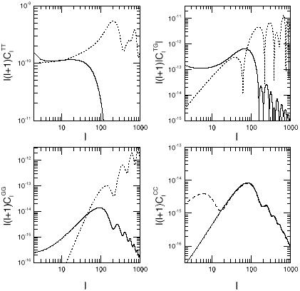
The power spectra can be computed for a given cosmological model through well-known numerical techniques. A set of power spectra for scalar and tensor perturbations in a typical inflation-like cosmological model, generated with the CMBFAST code (Seljak and Zaldarriaga, 1996) are displayed in Fig. 2.

Figure 2. Theoretical predictions for the four nonzero CMB temperature-polarization spectra as a function of multipole moment l. The solid curves are the predictions for a COBE-normalized scalar perturbations, while the dotted curves are COBE-normalized tensor perturbations. Note that the panel for ClC contains no dotted curve since scalar perturbations produce no ``C'' polarization component; instead, the dashed line in the lower right panel shows a reionized model with optical depth = 0.1 to the surface of last scatter.