


As discussed in the previous section, indications on the dominant stellar population can be easily derived even by simply comparing the observed data with the stellar spectra. More quantitative results can be obtained by comparing the absorption lines.
Several authors have used this method to classify the stars by their near-IR spectra (see references below). Usually two sets of lines are considered to derive both the spectral and the luminosity class, the first set depending both on temperature and gravity, while the second one on temperature only. The recipes used for star classification can also be applied to the observed galaxy spectra to derive indications on the the dominant stellar population.
We took into account two schemes of classification. They are both based on the CO(2,0) band head at 2.29 µm whose intensity depends both on temperature and luminosity and can be used to study the stellar populations in galaxies or in dusty regions (e.g., Armus et al., 1995; James & Seigar, 1999; Mobasher & James, 2000). The two methods use different thermometers: the first one, introduced by KH86 and refined by Ramirez et al. (1997), is based on the Equivalent Width (EW) of NaI 2.21µm and CaI 2.26µm which depend strongly on temperature but not on luminosity. In the second one, based on Origlia et al. (1993), the temperature is measured by the ratio of the two features at 1.62 and 1.59 µm. In both cases, the results for the galaxies are compared with those for the stars of known properties.
To apply these methods, we measured the EW of the lines with respect to a local continuum obtained by fitting a straight line to the "clear" parts of the spectrum. The spectral region used for both the line and the continuum are listed in Table 4. The same procedure was used to measure the EWs of the stars of the M98 and KH86. Because of the lower resolution of our spectra, our definitions are a little different from those by, for example, KH86 or Origlia et al. (1993), and the measured values of the EWs are consequently different. The errors on these quantities were estimated by taking into account both the noise of the spectra and the uncertainties in the continuum level. The latter contribution is usually the dominant one, especially in H where many features are present and it is difficult to define the continuum level. The results for the lines used in the classification are shown in Table 5 for the average ES spectra and in Table 6 for the individual galaxies not used for the templates. It should be noted that the error on the 1.62/1.59 ratio shown in the table is smaller than the error on each single line because the same continuum fit is used: the uncertainties on the continuum level strongly affect the measure of the EW of each line, but partially cancel out from their ratio.
| Feature | Line | Continuum |
| (µm ) | (µm) | |
| 1.59 | 1.586-1.594 | 1.572-1.574, 1.608-1.613 |
| 1.628-1.633 | ||
| 1.62 | 1.616-1.629 | 1.572-1.574, 1.608-1.613 |
| 1.628-1.633 | ||
| NaI | 2.204-2.211 | 2.191-2.197, 2.213-2.217 |
| CaI | 2.258-2.269 | 2.245-2.256, 2.270-2.272 |
| 12CO(2,0) | 2.289-2.302 | 2.270-2.272, 2.275-2.278 |
| 2.282-2.286, 2.288-2.289 | ||
| Feature | E+S0+Sa | Sb | Sc |
| 1.59 | 3.9 (0.8) | 3.7 (0.9) | 3.3 (0.9) |
| 1.62 | 6.0 (0.7) | 5.6 (0.8) | 5.7 (0.8) |
| 1.59/1.62 | 1.5 (0.1) | 1.5 (0.2) | 1.7 (0.2) |
| 12CO(2,0) | 14.6 (1.7) | 15.8 (1.7) | 15.6 (1.7) |
| CaI | 2.6 (1.1) | 2.7 (1.1) | 2.2 (1.1) |
| NaI | 3.4 (0.7) | 4.2 (0.7) | 3.4 (0.7) |
| NGC2798 | NGC1569 | NGC4449 | |
| 12CO(2,0) | 11.8 (2.4) | 16.7 (2.3) | 13.8 (2.9) |
| NaI+CaI | < 3.7 | < 4.2 | < 5.8 |
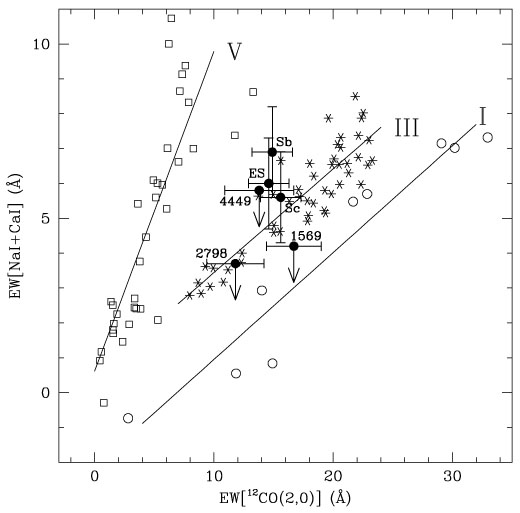
In Figure 12 we present the classification based on
the features in the K band studied by KH86 and
Ramirez et al. (1997).
This figure differs from both works because the feature definition is
different (because of the lower resolution) and because we don't take
into account the EW of
Br which cannot be reliably
measured. As expected, the results show that in all the cases the main role
is played by class III stars, possibly with some
contribution from dwarf stars. With the present data it does not seem
possible to measure this contribution and therefore constraint the ratio
between dwarf and giant stars, but this could be done with higher
resolution observations. The spectra of the active galaxies (see
Figure 4) are too
noisy to measure the EWs of NaI and CaI, and only upper limits can be
derived. As shown in Figure 12, these upper limits
put two of these galaxies in the region between class I and class III
stars, suggesting that the contribution supergiants
might be important in these galaxies.
which cannot be reliably
measured. As expected, the results show that in all the cases the main role
is played by class III stars, possibly with some
contribution from dwarf stars. With the present data it does not seem
possible to measure this contribution and therefore constraint the ratio
between dwarf and giant stars, but this could be done with higher
resolution observations. The spectra of the active galaxies (see
Figure 4) are too
noisy to measure the EWs of NaI and CaI, and only upper limits can be
derived. As shown in Figure 12, these upper limits
put two of these galaxies in the region between class I and class III
stars, suggesting that the contribution supergiants
might be important in these galaxies.
|
Figure 12. The sum of the EWs of NaI (2.21 µm) and CaI (2.26 µm) is plotted versus the EW of the 12CO(2,0) band at 2.29 µm. The solid dots with the error bars are our galaxies, while dwarf, giant and supergiant stars are plotted as empty squares, stars and empty circle respectively (see text for references). The lines are linear fit to the stellar data, with the indication of the luminosity class. |
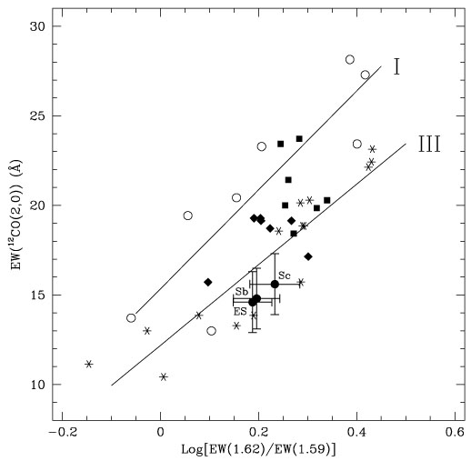
In Figure 13 we apply the second method based on the CO feature at 2.29µm and on the ratio of the 1.59 and 1.62µm in the H band. This method is based on the work by Origlia et al (1993) who showed that this ratio can be use as a thermometer in case of giants and supergiants stars. Also in this case the line ratio is consistent with the class III stars.
|
Figure 13. EW of the 12CO(2,0) feature at 2.29µm vs. the ratio EW(1.62)/EW(1.59). Giants and supergiants stars (see text for references) are plotted by empty circles and stars respectively. The galaxies observed by Origlia et al. (1993) are plotted by solid diamonds if quiescent ellipticals and spirals, and solid squares if HII galaxies. Solid circles with error bars 1are the galaxies of this study. The lines are the linear fit to the stellar data. |
A discussion about the metallicity of ellipticals and early spirals is
beyond the scope of this paper. Detail discussions about the information
of metallicity and element ratios based on optical data can be found, for
example, in
Worthey (1998) and
Trager et al. (2000).
Origlia et al. (1997)
have shown that moderate-resolution near-IR spectra can
also be used to measure the metallicity of the systems.
Their recipe is based on the 1.62µm feature which
is shown to depend on the metallicity index [Fe/H]
and, more weakly, on the carbon depletion factor [C/Fe].
It also depends on the microturbolent velocity
 of the dominant
stellar populations because this quantity influences the strength of the
saturated molecular lines. By observing globular clusters of known
metallicity,
Origlia et al. (1997)
show that this metallicity scale gives
errors smaller that 0.3 dex. These authors have also observed a limited
number of elliptical galaxies. The few metallicity estimates published
for these objects are based on the Mg2 index (see, for example,
Davies et al., 1987)
and on the Mg2-metallicity calibration by
Casuso et al. (1996).
While the Mg2-derived value of [Fe/H] of the observed
galaxies was solar or slightly supersolar, between +0.08 and +0.21,
the values based on the
near-IR lines turned out to be subsolar, between -0.28 and -0.46. This
can be explained either by the presence of a corresponding Magnesium
enhancement of about [Mg/Fe]
of the dominant
stellar populations because this quantity influences the strength of the
saturated molecular lines. By observing globular clusters of known
metallicity,
Origlia et al. (1997)
show that this metallicity scale gives
errors smaller that 0.3 dex. These authors have also observed a limited
number of elliptical galaxies. The few metallicity estimates published
for these objects are based on the Mg2 index (see, for example,
Davies et al., 1987)
and on the Mg2-metallicity calibration by
Casuso et al. (1996).
While the Mg2-derived value of [Fe/H] of the observed
galaxies was solar or slightly supersolar, between +0.08 and +0.21,
the values based on the
near-IR lines turned out to be subsolar, between -0.28 and -0.46. This
can be explained either by the presence of a corresponding Magnesium
enhancement of about [Mg/Fe]
 0.5, as proposed by several
authors (see
Origlia et al., 1997
for details), or by an anticorrelation between
[C/Fe] and [Fe/H], the more metallic objects being more carbon depleted, as
observed in the globular clusters. More recently, several authors
(Trager et al., 2000;
Worthey, 1998)
would rather explain the non-solar [Mg/Fe] with
a depletion of the iron-peak elements.
0.5, as proposed by several
authors (see
Origlia et al., 1997
for details), or by an anticorrelation between
[C/Fe] and [Fe/H], the more metallic objects being more carbon depleted, as
observed in the globular clusters. More recently, several authors
(Trager et al., 2000;
Worthey, 1998)
would rather explain the non-solar [Mg/Fe] with
a depletion of the iron-peak elements.
Despite the large uncertainties on the right value of [C/Fe]
and on the resulting metallicity, we have applied this method to our
early-type galaxies (ES spectrum, see table 5).
By iteratively solving the eq. 2 by
Origlia et al. (1997)
we obtain a mean microturbolent velocity
of about 3.1 km/sec,
in agreement with the values between 2.3 and 3.0 in
Origlia et al. (1997).
By using the 'standard' value of [C/Fe] = -0.3 suggested by these authors
and derived for the Magellanic Clouds clusters by
Oliva & Origlia (1998),
the metallicity derived from their eq. 1b is [Fe/H]
-0.20, reducing to [Fe/H]
-0.4 for [C/Fe] = 0.0.
The error on this quantity is difficult to estimate and is probably
dominated by the uncertainties on [C/Fe], but this result can be used as an
indication of sub-solar abundance of iron in the early-type galaxies.