Topological Defects in Cosmology

2.3. Cosmic strings

Cosmic strings are without any doubt the topological defect most thoroughly studied, both in cosmology and solid-state physics (vortices). The canonical example, also describing flux tubes in superconductors, is given by the Lagrangian

(7)

with F_µ = partial _[µ A_], where A is the gauge field and the covariant derivative is D_µ = partial _µ + i e A_µ, with e the gauge coupling constant. This Lagrangian is invariant under the action of the Abelian group G = U(1), and the spontaneous breakdown of the symmetry leads to a vacuum manifold curlyM that is a circle, S¹, i.e., the potential is minimized for phi = eta exp(i theta ), with arbitrary 0 leq theta leq 2. Each possible value of theta corresponds to a particular `direction' in the field space.

Figure 3. The complex scalar Higgs field evolves in a temperature-dependent potential V( phi ). At high temperatures (violet surface) the vacuum expectation value of the field lies at the bottom of V. For lower temperatures, the potential adopts the "Mexican hat" form (yellow surface) and the field spontaneously chooses one amongst the new available (degenerate) lowest energy states (the violet circle along the valley of the hat). This isolates a single value/direction for the phase of the field, spontaneously breaking the symmetry possessed by the system at high energies. Different regions of the universe, with no causal connection, will end up having arbitrarily different directions for the field (arrows on the right). As separate regions of broken symmetry merge, it is not always possible for the field orientations to match. It may happen that a closed loop in physical space intersects regions where the Higgs phase varies from 0 to 2 (red arrows, corresponding to the red dashed-line on the left panel). In that situation, a cosmic string will pass somewhere inside the loop. On the contrary, green arrows (and green dashed-line on the left panel) show a situation where no string is formed after the phase transition.

Now, as we have seen earlier, due to the overall cooling down of the universe, there will be regions where the scalar field rolls down to different vacuum states. The choice of the vacuum is totally independent for regions separated apart by one correlation length or more, thus leading to the formation of domains of size ~ ^-1. When these domains coalesce they give rise to edges in the interface. If we now draw a imaginary circle around one of these edges and the angle varies by 2 then by contracting this loop we reach a point where we cannot go any further without leaving the manifold . This is a small region where the variable is not defined and, by continuity, the field should be = 0. In order to minimize the spatial gradient energy these small regions line up and form a line-like defect called cosmic string.

The width of the string is roughly m^-1 ~ (^1/2 )^-1, m being the Higgs mass. The string mass per unit length, or tension, is µ ~ ². This means that for GUT cosmic strings, where ~ 10¹⁶ GeV, we have Gµ ~ 10^-6. We will see below that the dimensionless combination Gµ, present in all signatures due to strings, is of the right order of magnitude for rendering these defects cosmologically interesting.

There is an important difference between global and gauge (or local) cosmic strings: local strings have their energy confined mainly in a thin core, due to the presence of gauge fields A_µ that cancel the gradients of the field outside of it. Also these gauge fields make it possible for the string to have a quantized magnetic flux along the core. On the other hand, if the string was generated from the breakdown of a global symmetry there are no gauge fields, just Goldstone bosons, which, being massless, give rise to long-range forces. No gauge fields can compensate the gradients of this time and therefore there is an infinite string mass per unit length.

Just to get a rough idea of the kind of models studied in the literature, consider the case G = SO(10) that is broken to H = SU(5) × curly Z ₂. For this pattern we have ₁( curlyM ) = curly Z ₂, which is clearly non trivial and therefore cosmic strings are formed [Kibble et al., 1982]. ⁽¹⁰⁾

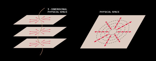
Figure 4. We can now extend the mechanism shown in the previous figure to the full three-dimensional space. Regions of the various planes that were traversed by strings can be superposed to show the actual location of the cosmic string (left panel). The figure on the right panel shows why we are sure a string crosses the plane inside the loop in physical space (the case with red arrows in the previous figure). Continuity of the field imposes that if we gradually contract this loop the direction of the field will be forced to wind "faster". In the limit in which the loop reduces to a point, the phase is no longer defined and the vacuum expectation value of the Higgs field has to vanish. This corresponds to the central tip of the Mexican hat potential in the previous figure and is precisely the locus of the false vacuum. Cosmic strings are just that, narrow, extremely massive line-like regions in physical space where the Higgs field adopts its high-energy false vacuum state.

¹⁰ In the analysis one uses the fundamental theorem stating that, for a simply-connected Lie group G breaking down to H, we have ₁(G / H) appeq ₀(H); see [Hilton, 1953]. Back.