Annu. Rev. Astron. Astrophys. 1999. 37: 487-531 Copyright © 1999 by Annual Reviews. All rights reserved

3.2. General Abundance Analysis

Abundance estimates from absorption lines are, in principle, more straightforward than for emission lines because the absorption strengths are not sensitive to the temperatures or space densities in the gas. Moreover, absorption lines yield direct measures of the column densities in different ions. We need only apply appropriate ionization corrections to convert the column densities into relative abundances. For example, the abundance ratio of any two elements a and b can be written,

(10)

which is identical to Equation 8 except that the Ns here are the column densities. Once again we define the ionization correction as IC log(f (b_j) / f (a_i)). Abundance studies would ideally compare lines with similar ionizations to minimize IC and reduce the sensitivity to potentially complex geometries. Unfortunately, the lines available often require significant ionization corrections. In particular, we are often forced to compare highly ionized metals (such as CIV) to HI (Ly) to derive the metallicity. We must therefore use ionization models.

The usual assumption is that the gas is photoionized by the QSO continuum flux. Collisional ionization would lead to lower derived metallicities because it creates less HI (and more HII) for a given level of ionization in the metals (cf Figures 4 and 5 in Hamann et al. 1995; see also Turnshek et al. 1996). However, collisional ionization has been generally dismissed for BAL regions (BALRs) because (a) it would be energetically hard to maintain, (b) it would produce excessive amounts of line emission (because of the much higher temperatures), and (c) it is hard to reconcile with the observed simultaneous variabilities in BAL troughs across a wide range of velocities (Weymann et al. 1985, Junkkarinen et al. 1987, Barlow 1993). In contrast, the strong radiative flux known to be present in QSOs provides a natural ionization source. We will assume that photoionization dominates in both BALRs and intrinsic NALRs.

Estimates of IC generally come from plots like Figure 10, which shows the ionization fractions of HI and various metal ions M_i in photoionized clouds (see Section 2.5 and Ferland et al. 1998 for general descriptions of the calculations). Ideally, we would compare column densities in different ions of the same element to obtain abundance-independent constraints on the ionization and thus IC. Otherwise, column densities in different elements can also constrain IC with assumptions about their relative abundances.

Figure 10. Ionization fractions in optically thin clouds photoionized by a power-law spectrum with = -1.5. Results are shown for a range of ionization parameters, U (see Section 2.5.1). The HI fraction appears across the top. The curves for the metal ions are labeled above or below their peaks whenever possible. The notation here is HI = H0, CIV = C+3 etc.

Note that the results in Figure 10 are not sensitive to the particular abundances used in the calculations (in this case solar), so the figure is useful for general abundance/ionization estimates (see Hamann 1997). The model clouds are optically thin in the ionizing UV continuum, which means that gradients in the ionization are negligible across the cloud and the ionization fractions do not depend on the total column densities. This simplification appears to be appropriate for most intrinsic absorption line systems (based on their measured column densities), although shielding by many far-UV BALs might affect the ionization structure downstream in BALRs (Korista et al. 1996, Turnshek 1997, Hamann 1997). Also, systems with low-ionization lines like FeII or MgII can be optically thick at the HI Lyman edge (Bergeron & Stasinska 1986, Voit et al. 1993, Wampler et al. 1995) and may require calculations with specific column densities that match the data.

3.2.1. Ionization Ambiguities

The main theoretical uncertainties involve the shape of the ionizing spectrum, the frequent lack of ionization constraints (too few lines measured), and the possibility of inhomogeneous (multizone) absorbing regions. Hamann (1997) addressed these issues by calculating IC values for a wide range of conditions in photoionized clouds. He noted that, whenever there is or might be a multizone absorber with a range of ionization states, we can still make conservatively low estimates of the metal-to-hydrogen abundance ratios by assuming each metal line forms where that ion is most favored - that is, at the peak of its ionization fraction f(M_i) in Figure 10. We can also place firm lower limits on the metal-to-hydrogen ratios by adopting the minimum values of IC, which correspond to minima in the f(HI) / f(M_i) ratios (see also Bergeron & Stasinska 1986). The lower limits are robust, even though they come from one-zone calculations, because the presence of different or additional zones can only mean that larger IC values are appropriate for the data. Figure 11 plots several minimum metal-to-hydrogen ICs for optically thin clouds photoionized by different power-law spectra. The results in this plot simply get added to the logarithmic column density ratios (Equation 10) to derive minimum metallicities. Note that some important metal-to-metal ratios also have minimum IC values, such as PV/CIV and FeII/MgII (Hamann 1998; F Hamann, R Chaffee, RJ Weymann, TA Barlow, VT Junkkarinen, manuscript in preparation).

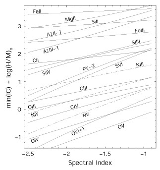Figure 11. Minimum metal ion-to-HI ionization corrections (IC) normalized to solar abundances (the last two terms in Equation 10) are plotted for optically thin clouds photoionized by power-law spectra with different indices (). The notation is the same as Figure 10. The curves have been shifted vertically by +1 for OVI, by -2 for PV, and by -1 for AlII and AlIII. The curves for nitrogen ions are dash-dot.

3.2.2. Column Densities and Partial Coverage

The final critical issue is deriving accurate column densities from the absorption troughs. In the simplest case, the optical depths in well-resolved lines are related to the observed intensities by,

(11)

where I_v and I_o are the observed and intrinsic (unabsorbed) intensities, respectively, and _v is the line optical depth, at each velocity shift v. The column densities follow from the optical depths by,

(12)

where f is the oscillator strength and _o is the laboratory wavelength of the line. Column density derivations can involve line profile fitting or direct integration over the observed profiles (via Equations 11 and 12, Junkkarinen et al. 1983, Grillmair & Turnshek 1987, Korista et al. 1992, Savage & Sembach 1991, Jenkins 1996, Arav et al. 1999). Very optically thick lines are not useful because the inferred values of _v are far too sensitive to uncertainties in I_v. In other cases, the analysis might still be compromised by (a) unresolved absorption line components or (b) unabsorbed flux that fills in the bottoms of the observed troughs. If either of these possibilities occurs, the derived optical depths and column densities become lower limits, and the derived abundances become incorrect. Errors from the first possibility can always be reduced or avoided by higher-resolution spectroscopy.

The second possibility, of filled-in absorption troughs, is actually an asset for identifying intrinsic NALs (Section 3.1). We refer to this filling-in generally as partial coverage of the background emission source(s). Figure 12 shows several geometries that might produce partial coverage and filled-in troughs. ⁽³⁾ (The situation can be potentially more complicated if the absorber itself is a source of emission. The analysis discussed below remains the same, however.) When partial coverage occurs, the observed intensities depend on both the optical depth and the line-of-sight coverage fraction, C_f, at each velocity,

(13)

where 0 C_f 1, and the first term on the right side is the unabsorbed (or uncovered) contribution. Measured absorption lines can thus be shallow even when the true optical depths are large. In the limit _v >> 1, we have

(14)

Outside of that limit, we can compare lines whose true optical-depth ratios are fixed by atomic physics, such as the HI Lyman lines or doublets like CIV 1548,1550, SiIV 1394,1403 etc, to determine uniquely both the coverage fractions and the true optical depths across the line profiles (Hamann 1997b, Barlow & Sargent 1997, Arav et al. 1999, Srianand & Shankaranarayanan 1999, Ganguly et al. 1999). For example, a little algebra shows that for doublets with true optical-depth ratios of ~ 2 (as in CIV, SiIV, etc), the coverage fraction at each absorption velocity is,

(15)

where I₁ and I₂ are the observed line intensities, normalized by I_o, at the same velocity in the weaker- and stronger-line troughs, respectively. The corresponding line optical depths are ₂ = 2₁ and

(16)

Figure 12. Possible "partial-coverage" geometries. Partial line-of-sight coverage occurs when light rays like C, which pass through absorption line clouds (indicated by filled ellipsoids), are combined with rays like A, B, or D, which do not. Ray A represents reflected light from a putative scattering region. Ray B simply misses the absorption line region. Ray D passes through the nominal absorbing zone but suffers no absorption because the region is porous.

The only drawback of partial coverage for the NALs is that there might be a range of coverage fractions in multizone-absorbing media. There is already evidence in some cases for coverage fractions that differ between ions or change with velocity across the line profiles (Barlow & Sargent 1997, Barlow et al. 1997, Hamann et al. 1997b). Variations in C_f with velocity can always be dealt with by analyzing limited velocity intervals in the line profiles (see also Arav 1997). But one can imagine complex geometries where ionization-dependent coverage fractions would jeopardize the simple abundance analysis described above, in particular for comparisons between high- and low-ionization species like CIV and HI. Abundance ratios based on disparate species like these might require specific models of the ionization-dependent coverage. On the other hand, this worst-case scenario is not known to occur, and there is no reason to believe it would lead to generally overestimated metallicities anyway.

³ The situation can be potentially more complicated if the absorber itself is a source of emission. The analysis discussed below remains the same, however. Back.