Annu. Rev. Astron. Astrophys. 1980. 18: 165-218 Copyright © 1980 by Annual Reviews. All rights reserved

3. PHYSICAL PARAMETERS

In the early treatizes on this subject, the mean value assigned to it will be found to be 40.000000. Later writers suspected that the decimal point had been accidentally shifted, and that the proper value was 400.00000.

Lewis Carroll, "The new method of evaluation as applied to "
from Notes by an Oxford Chiel

Total intensity and polarization data can be used to extract information about several physical parameters intrinsic to radio sources and thereby help place constraints on some of the mechanisms involved. Since the advent of computers and more recently of pocket calculators, this "interpretation of the data" has become such an automatic ritual that the many assumptions inherent in each step are sometimes forgotten. We shall review here some of the arguments most commonly used in deriving physical parameters from intensity and polarized brightness distributions. In order to make the uncertainties more explicit, the formulas will be expressed as much as possible in terms of observed quantities. For block diagrams of the various steps and assumptions that are made the reader is referred to Miley (1976).

3.1. Total Intensity Distributions

3.1.1 ENERGETICS The energetics of radio sources are important not only because of their relation to the source-production mechanism but because they also play an important role in all considerations of how radio sources are held together or confined. Total intensity distributions provide information about the minimum energies involved. A good discussion of source energetics is given by Moffet (1975) and in more detail by Pacholcyzk (1970). The minimum energy condition corresponds almost (but not quite) to equipartition of energy between relativistic particles and magnetic field.

For a region in a synchrotron radio source delineated by an ellipse of angular diameters _x and _y in orthogonal directions, we can write the minimum energy density as

(1)

where the corresponding magnetic field is

(2)

Here k is the ratio of energy in the heavy particles to that in the electrons, is the filling factor of the emitting regions, z is the redshift, _x and _y (arcsec) correspond either to the source/component sizes or to the equivalent beam widths, s (kiloparsec) is the path length through the source in the line of sight, is the angle between the uniform magnetic field and the line of sight, F₀ (Jy or Jy per beam) is the flux density or brightness of the region at frequency ₀ (GHz), ₁ and ₂ (GHz) are the upper and lower cut off frequencies presumed for the radio spectrum, and is the spectral index [F() , ₁ < < ₂].

Apart from the basic assumptions that the radiation is synchrotron emission and that the radio and optical emission are redshifted by the same amount there are several more mundane uncertainties inherent in these formulas.

First, k is unknown and could have a value between 1 and 2000 (Pacholczyk 1970). Indirect arguments have usually led to canonical values of k = 1 or k = 100 (eg. Moffet 1975). k = 1 is clearly more consistent with the use of the minimum energy condition. Note that a difference of 100 in the assumed k results in an order-of-magnitude difference in the minimum energy densities derived. Second, to obtain s, the path through the source along the line of sight, one must make some assumptions about the symmetry and distance of the source. Frequently cylindrical symmetry is assumed, with s equal to the width of the source in the plane of the sky. Third, the formulas depend on the form of the source spectrum, but this dependence is weak. For extended sources -0.6, and ₁ dominates over ₂. Usually ₁ = 0.01 GHz is assumed. Fourth, the term is unknown in individual cases. It arises because the emission measure depends on the perpendicular component of the magnetic field and the visible radiation is beamed from electrons moving towards us. Fifth, and perhaps most irritating, is the strong dependence on the filling factor. It is possible that on a scale much less than an arcsecond or a kiloparsec the radiation is clumpy or filamentary. This would result in much greater local energy densities and less total energy.

Taking k = 1, = 1, sin = 1, ₁ = 0.01 GHz, ₂ = 100 GHz, = -0.8 we obtain approximate expressions for the minimum energy condition,

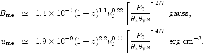
(3) (4)

The minimum energy condition is particularly sensitive to angular size. Because of the limited range of brightnesses that can be studied with a particular instrument, values of B_me derived from measurements made with the same telescope usually do not differ by much more than a factor of four or five. Typical values obtained for B_me are ~ 10^-6.5 for cluster halos, 10^-5.5 G for the diffuse lobes, ~ 10^-5 G for the hot spots, and ~ 10^-3 G for the tiny flat spectrum cores. Resultant total source energies can reach 10⁶⁰ ergs. However, it must be stressed that there is little evidence that the minimum energy condition is actually obeyed.

3.1.2 SOURCE CONFINEMENT In order to account for the nonspherical shapes of radio sources the particles and field must be prevented from dispersing at the relativistic internal sound speed of c / 3. The pressure exerted by the relativistic gas in the radio source, u/3, must therefore be balanced by some pressure, P, or by inertial drag. Several mechanisms have been considered for confinement (see, for example, Longair et al. 1973, Pacholczyk 1977) and in each case the pressure balance condition can be used to calculate limits for the various parameters that characterize the resisting forces.

Some possible confining mechanisms are listed in Table 1 together with the restrictions implied by pressure balance. Their applicability to the various regions of radio sources will be considered in Section 4. In real life several of these processes may be occurring simultaneously, and the detailed hydrodynamic interactions will probably result in a considerably more complicated situation than can be treated by simple static-pressure balance arguments.

v_t

Table 1. Some possible confinement mechanisms

	Mechanism	Approximate Restriction
Internal:	Gravitational: Point mass M at center of spherical source, diam. distance D (Mpc)	M 7 × 107 (D)2 Bme M
	(arcsec),
	Inertial: Blob, translational velocity, Source separation/component size, R/r	int 3 × 10-22(R/r)2 Bme2(vt / c)-2 gm cm-3
External:	Static thermal: Temperature T	ext T 2.5 × 10-10 Bme2 gm cm-3 deg
	Dynamic: Ram pressure, translational velocity vt	ext 7 × 10-23 Bme2(vt / c)-2 gm cm-3
	Magnetic	Bext Bme

3.1.3 MAGNETIC FIELD FROM COMPARISON WITH X RAYS An independent method of obtaining information about the distribution of magnetic field strengths in extended sources is based on the fact that the same relativistic electrons that produce the radio synchrotron emission will scatter photons of the microwave background to X rays. The ratio between radio and X-ray surface brightness depends on the magnetic field strength (Perola & Reinhardt 1972, Bridle & Feldman 1972, Costain et al. 1972, Harris & Romanishin 1974, Harris & Grindlay 1979). The process is reviewed by Gursky & Schwartz (1977).

The expression for the resultant magnetic field strength given by Harris & Grindlay (1979) can be approximated to within about ± 10% between -0.6 > > -1.4 and rewritten as

(5)

where F_R is the radio flux density (in Jy) at frequency _R (GHz), F_x is the X-ray flux (erg cm^-2 Hz^-1) at energy E_x (keV), is the spectral index (F_{R R}) and z is the redshift.

The main problems in using this method to determine the magnetic field strengths in extended radio sources arise from the required X-ray surface brightness sensitivity and the difficulty of separating possible inverse Compton X rays from the thermal X-ray distribution. However, one can at least obtain an upper limit for the inverse Compton contribution and hence a lower limit on the magnetic field strengths. Until now this has been done using only a few relatively low resolution X-ray measurements. For Centaurus A Cooke et al. (1978) obtained B 7 × 10^-7 G and for Cygnus A Fabbiano et al. (1979) obtained B 1.6 × 10^-6 G indicating that the extended lobes are not too far from equipartition. With high sensitivity X-ray observations and resolution comparable to the radio maps, this method promises to provide more information about magnetic fields in extended radio sources. A beginning is now being made with the Einstein Observatory, which, although providing an enormous improvement in X-ray sensitivity and resolution, can detect extended inverse Compton emission only from a few of the strongest sources.

3.1.4 AGES - IN SITU ACCELERATION A problem frequently considered in discussions of source morphology concerns the place where the observed synchrotron electrons are accelerated. Does this occur entirely in the nucleus, mainly in the hot spots, or is there an accelerating process at work throughout the entire source?

For the acceleration to have taken place at an angular distance (arcsec) from where the radiation is observed, the electron must have traveled to its present position in time,

(6)

where D (Mpc) is the "angular size" distance (McVittie 1965), v (km s^-1) is the velocity at which electrons travel from the nucleus to the position under study, is the angle between this direction and the line of sight. For an isotropic distribution of pitch angles the average age of a radiating synchrotron electron, t_r, is (van der Laan & Perola 1969, De Young 1976)

(7)

where B (G) is the magnetic field strength in the source, B_R = 4 × 10^-6(1 + z)² G is the equivalent magnetic field strength of the microwave background. _* (GHz) is the frequency above which an exponential drop in flux will occur, and usually exceeds ₀, the observing frequency. A necessary condition for acceleration to have occurred at a distance is t_d = t_r, i.e.

(8)

To apply this condition we need to have some information about v and B. Of course we can always take v < c, but in most cases there is evidence that the velocities are considerably smaller. If we accept the radio-trail hypothesis (Section 2.2.1), for tailed sources v is the velocity of the parent galaxy. A reasonable upper limit to v of a few thousand km s^-1 is then given by the distribution of radial velocities of galaxies in the cluster. Likewise, for the lobes of double sources, the observed asymmetry has been used as a statistical argument that the outward electron velocities are smaller than 0.2 c (Sections 4.2 and 4.4). An additional possible upper limit to the velocities is the generalized sound speed in the source (u / )^1/2 which in the equipartition case reduces to the Alfvén velocity B/(4 )^1/2, However, this is less certain since resonant damping by thermal protons in the source might permit considerably higher velocities (Holman et al. 1979).

There are two ways of specifying B. The first is to assume that the minimum energy (~ equipartition) condition holds and to calculate B from (2) or (3). The weaknesses of this approach are the lack of evidence for equipartition and the uncertainties in the formulas. (Note that minimum energy does not imply minimum B.) Also, the assumption that the pitch angles are isotropically distributed may be invalid. In that case one must replace B by B = B sin, so electrons flowing along the magnetic field lines will suffer smaller energy losses and have prolonged lives (Spangler 1979).

One can avoid most of these limitations by choosing B = B_R / 3, the value that gives a maximum radiative lifetime (van der Laan & Perola 1969). The necessary condition for remote acceleration then becomes

(9)

In Section 4 evidence will be presented that localized particle acceleration in radio sources may be widespread and almost certainly occurs in jets where optical emission has been seen. An imaginative assortment of complicated mechanisms has been invoked to produce this in situ acceleration (see, for example, Pacholczyk & Scott 1976, Lacombe 1977, Blandford & Ostriker 1978, Eichler 1979, Eilek 1979, Ferrari et al. 1979, Smith & Norman 1979), but in view of the many assumptions and free parameters inherent in these models, they will not be discussed here.