

8.2. Cross Correlation
A main aim of studying the line and continuum light curves is to measure the "BLR size". This quantity may be defined in several different ways. For example, an emissivity-weighted average radius, rav, is defined by

| (71) |
Other measures of the "BLR size" are mentioned below.
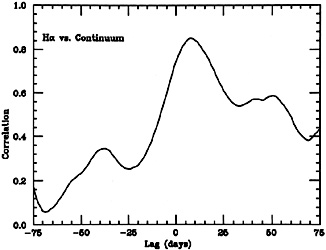
Cross correlating the line and continuum light curves is a simple way of estimating the dimension of the line emitting region. This is a well known technique, designed to give the most likely time-lag between the line and continuum pulses. The Cross Correlation Function (CCF) is a set of correlation coefficients, giving a measure of the correlation between the line and continuum light curves for certain chosen time lags. Fig. 18 shows the CCF for the two light curves of NGC 4151. A clear broad, significant peak (a correlation coefficient of 0.85 for 55 points) is seen at a lag of 9 days. This time lag, multiplied by c, can be defined as "the cross-correlation size" of the BLR.
There are several problems in applying the cross correlation method to real data sets. Some interpolation is required in order to use this procedure for unevenly sampled light curves. This can be disastrous in cases of large gaps in the data and/or short data strings. Observational errors can also affect the position of the CCF peak. As a general rule, the mean sampling interval must be considerably shorter than the typical continuum variability time scale. This reduces the interpolation errors and the resulting uncertainty in the position of the peak. Finally, the cross-correlation peak position depends on the nature of the continuum light curve and the response (linear or non-linear) of the lines. Thus the above mentioned "cross-correlation size", obtained from the CCF of one emission line, is not very well defined.

|
Figure 18. The cross-correlation function
of H |
A serious limitation of the cross correlation analysis is the lack of a solid criterion for estimating its uncertainty. Some formulaebservations. Here, again, the meaning of the derived time-lag uncertainty is somewhat ambiguous.
A main disadvantage of the cross correlation method is the fact that the entire data set, sometimes the result of one or two observing seasons, is used to obtain one number (the time lag). Weather, telescope scheduling and other limitations result in a random sampling of the intrinsic light curve which, if sampling is not frequent enough, means an uncertain result. Many more experiments, of similar duration, must in principle be performed in order to asses the accuracy of such results. This is not practical and numerical simulations, mimicking the real observing conditions, are used instead. One method developed for this purpose utilizes Monte-Carlo simulations to find the Cross Correlation Peak Distribution (CCPD) which gives the probability of finding the peak of the CCF at a certain lag, given an assumed continuum light curve and a certain geometry. Obviously, the CCPD is narrower, and the results more meaningful, for cases of frequent sampling and high signal/noise data.
Finally, the time lag obtained from the peak of the CCF is not necessarily a good indicator of the gas distribution, even for well sampled light curves. It tends to weight the inner parts of the line emission region more than the outer parts, in a way which depends on the continuum light curve. For thick geometries, the cross-correlation size is considerably smaller than the emissivity-weighted radius, rav of (71).