Annu. Rev. Astron. Astrophys. 1998. 36: 17-55 Copyright © 1998 by Annual Reviews. All rights reserved

5. H₀ FROM PHYSICAL CONSIDERATIONS

To first order, there is a natural SN Ia peak luminosity - the instantaneous radioactivity luminosity, i.e. the rate at which energy is released by ⁵⁶Ni and ⁵⁶Co decay at the time of maximum light (Arnett 1982, Arnett et al 1985, Branch 1992). With certain simplifying assumptions, the peak luminosity is predicted to be identical to the instantaneous radioactivity luminosity. The extent to which they differ, for a hydrodynamical explosion model, can be determined only by means of detailed light curve calculations that take into account the dependence of the opacity on the composition and the physical conditions. The state of the art is represented by the calculations of Höflich & Khokhlov (1996). The calculated peak luminosity of the models turns out to be proportional to M_Ni within uncertainties, and for models that can be considered to be in the running as representations of normal SNe Ia (carbon ignitors that take longer than 15 days to reach maximum light in the V band), the characteristic ratio of the peak luminosity to the radioactivity luminosity is about 1.2 (Branch et al 1997). The physical reason that the ratio exceeds unity in such models was explained by Khokhlov et al (1993) in terms of the dependence of the opacity on the temperature, which is falling around the time of maximum light.

Höflich & Khokhlov's (1996) light-curve calculations can be used to estimate H₀ in various ways. Höflich & Khokhlov (1996) themselves compared the observed light curves of 26 SNe Ia (9 in galaxies having radial velocities greater than 3000 km s^-1) to their calculated light curves in two or more broadbands, to determine the acceptable model(s), the extinction, and the distance for each event. From the distances and the parent-galaxy radial velocities, they obtained H₀ = 67 ± 9. Like the empirical MLCS method, this approach has the attractive feature of deriving individual extinctions. But identifying the best model(s) for a SN while simultaneously extracting its extinction and distance, all from the shapes of its light curves, is a tall order. This requires not only accurate calculations but also accurate light curves, and the photometry of some of the SNe Ia that were used by Höflich & Khokhlov (1996) has since been revised (Patat et al 1997). And because Höflich & Khokhlov's (1996) models included many more underluminous than overluminous SNe (the former being of interest in connection with weak SN Ia like SN 1991bg) while the formal light-curve fitting technique has a finite "model resolution," a bias towards deriving low luminosities and short distances for the observed SNe Ia is possible.

There are less ambitious but perhaps safer ways to use Höflich & Khokhlov's (1996) models to estimate H₀ that involve an appeal to the homogeneity of normal SNe Ia and rely only on the epoch of maximum light when both the models and the data are at their best. The 10 Chandrasekhar-mass models having 0.49 M_Ni 0.67 - i.e. those having M_Ni within the acceptable range for normal SNe Ia - have a mean M_Ni = 0.58 M and a mean M_V = -19.44. Alternatively, the five models (W7, N32, M35, M36, PDD3) that Höflich & Khokhlov (1996) found to be most often acceptable for observed SNe Ia have a mean M_Ni = 0.58 and a mean M_V = -19.50. Using M_V = -19.45 ± 0.2 in Equation 1 gives H₀ = 56 ± 5, neglecting extinction of the non-red Hubble-flow SNe Ia.

Höflich & Khokhlov's (1996) light-curve calculations were used in another way by van den Bergh (1995). Noting that the maximum light M_V and B - V values of the models obey a relation that mimics that which would be produced by extinction (Figure 15), he matched the model relation between M_V and B - V to the relation of the observed Hubble-flow SN Ia and obtained values of H₀ in the range of 55-60, depending on how the models were weighted. If helium-ignitor models had been excluded, the resulting H₀ would have been a bit lower because the models are underluminous for their B - V colors. This procedure has the virtue of needing no estimates of extinction. The same result can be seen from figure 3 of Höflich et al (1996), who plotted M_V versus B - V for Höflich & Khokhlov (1996) models and for the Calán-Tololo SNe Ia. For the assumed value of H₀ = 65, the relations between M_V and B - V for the models and the observed SNe Ia are offset, and H₀ would need to be lowered to about 55 to bring them into agreement.

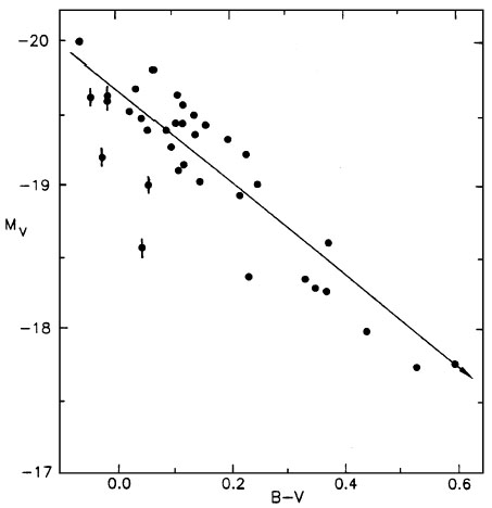Figure 15. MV is plotted against B - V for the models of Höflich & Khokhlov (1996). Helium-ignitor models are indicated by vertical lines. The arrow has the conventional extinction slope of 3.1. Adapted from van den Bergh (1996).

In their Figure 2, Höflich et al (1996) also plot M_V versus a V-band light-curve decline parameter that is analogous to m₁₅, for the models and for the Calán-Tololo SNe Ia. Again with H₀ = 65, the models and the observed SNe I are offset, with H₀ needing to be lowered to about 55 to bring them into agreement.

Distances to SNe Ia also can be derived by fitting detailed NLTE synthetic spectra to observed spectra. Nugent et al (1995b) used the fact that the peak luminosities inferred from radioactivity-powered light curves and from spectrum fitting depend on the rise time in opposite ways, in order to simultaneously derive the characteristic rise time and luminosity of normal SNe Ia and obtained H₀ = 60⁺¹⁴_-11. If SN Ia atmospheres were not powered by a time-dependent energy source, the spectrum-fitting technique could be independent of hydrodynamical models. The procedure would be to look for a model atmosphere that accounts for the observed spectra without worrying about how that atmosphere was produced, estimate (or derive by fitting two or more phases) the time since explosion, and obtain the luminosity of the model. But, owing to the time-dependent nature of the deposition of radioactivity energy, SNe Ia "remember" their history (Eastman 1997, Nugent et al 1997, Pinto 1997). Light-curve and spectrum calculations really are coupled, and more elaborate physical modeling needs to be done.