5.2. Missing Metals?

It can also be appreciated from Figure 32 that our knowledge of element abundances at high redshift is still very patchy. This becomes all the more evident when we attempt a simple counting exercise. Figure 33 shows a recent version of a plot first constructed by Madau et al. (1996) which attempts to trace the `cosmic star formation history' by following the redshift evolution of the comoving luminosity density of star forming galaxies. This kind of plot enjoyed great popularity after it was presented by Madau et al.; more recently astronomers have approached it with greater caution as they have become more aware of the uncertainties involved. In particular, the dust corrections to the data in Figure 33 have been the subject of intense debate over the last five years, as has been the contribution to _* from galaxies which may be obscured at visible and ultraviolet wavelengths and only detectable in the sub-mm regime with instruments such as SCUBA. Furthermore, the normalisation of the plot depends on the IMF and on the slope of the faint end of the galaxy luminosity function. Nevertheless, if we assume that we have the story about right, some interesting consequences follow.

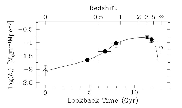Figure 33. The comoving star formation rate density * vs. lookback time compiled from wide angle, ground based surveys (Steidel et al. 1999 and references therein). The data shown here are for a H0 = 50 km s-1 Mpc-1, M = 1, = 0 cosmology.

The first question one may ask is: "What is the total mass in stars obtained by integrating under the curve in Figure 33?" The data points in Figure 33 were derived assuming a Salpeter IMF (with slope -2.35) between M = 100 M and 0.1 M. However, for a more realistic IMF which flattens below 1 M, the values of _* in Figure 33 should be reduced by a factor of 2.5. ⁽²⁾ With this correction:

(5.7)

where _crit = 3.1 × 10¹¹ h² M Mpc^-3 and _stars (1.5 - 3) h^-1 × 10^-3 (Cole et al. 2001) is the fraction of the closure density contributed by stars at z = 0. Thus, within the rough accuracy with which this accounting can be done, the star formation history depicted in Figure 33 is apparently sufficient to produce the entire stellar content, in disks and spheroids, of the present day universe. Note also that 1/4 of today's stars were made before z = 2.5 (the uncertain extrapolation of _* beyond z = 4 makes little difference).

We can also ask: "What is the total mass of metals produced by z = 2.5?". Using the conversion factor _metals = 1/42 _* to relate the comoving density of synthesised metals to the star formation rate density (Madau et al. 1996) we find

(5.8)

which corresponds to

(5.9)

where _baryons = 0.088 for h = 0.5 (Section 1.1) and 0.0189 is the mass fraction of elements heavier than helium for solar metallicity (Grevesse & Sauval 1998). In other words, the amount of metals produced by the star formation we see at high redshift (albeit corrected for dust extinction) is sufficient to enrich the whole baryonic content of the universe at z = 2.5 to 1/30 of solar metallicity. Note that this conclusion does not depend sensitively on the IMF.

As can be seen from Table 3, this leaves us with a serious `missing metals' problem which has also been discussed in more detail by Pagel (2002). The metallicity of damped Ly systems is in the right ballpark, but _DLA is only a small fraction of _baryons. Conversely, while the Ly forest may account for a large fraction of the baryons, its metal content is one order of magnitude too low. The contribution of Lyman break galaxies to the cosmic inventory of metals is even more uncertain. The value in Table 3 is a strict (and not very informative) lower limit, calculated from the luminosity function of Steidel et al. (1999), taking into account only galaxies brighter than L^* and assigning to each a mass M^* = 10¹¹ M (which is likely to be a lower limit, as discussed by Pettini et al. 2001) and metallicity Z = 1/3 Z. Galaxies fainter than L^* are not included in this census because we still have no idea of their metallicities; potentially they could make a significant contribution to _Z(LBG) because they are so numerous.

Table 3. Census of Metals at z = 2.5 ^a

Component	b	Z c	Z d
Observed :
DLAs	0.0025	0.07	0.002
Ly Forest	0.05 - 0.08	0.003	0.002 - 0.003
Lyman Break Galaxies	?	0.3	> 0.0002
Predicted :
All Baryons (BBNS)	0.088
Metals synthesised in
Lyman Break Galaxies			0.035
a All entries are for H0 = 50 km s-1 Mpc-1 ; M = 1, = 0. b In u nits of the closure density crit = 3.1 × 1011 h2 M Mpc-3. c In units of solar metallicity (0.0189 by mass). d In units of Z = baryons × Z = 1.7 × 10-3.

Nevertheless, when we add up all the metals which have been measured with some degree of confidence up to now, we find that they account for no more than 10 - 15% of what we expect to have been produced by z = 2.5 (last column of Table 3). Where are these missing metals? Possibly, _Z(DLA) has been underestimated, if the dust associated with the most metal-rich DLAs obscures background QSOs sufficiently to make them drop out of current samples. However, preliminary indications based on the CORALS survey by Ellison et al. (2001) suggest that this may be a relatively minor effect (see also Prochaska & Wolfe 2002). The concordance in the values of _Z(IGM) derived from observations of O VI and C IV absorption in the Ly forest makes it unlikely that the metallicity of the widespread IGM has been underestimated by a large factor. On the other hand, we do know that Lyman break galaxies commonly drive large scale outflows; it is therefore possible, and indeed likely, that they enrich with metals much larger masses of gas than those seen directly as sites of star formation. This gas and associated metals may be difficult to detect if they are at high temperatures, and yet may make a major contribution to _Z; there are tantalising hints that this could be the case at the present epoch (Tripp, Savage, & Jenkins 2000; Mathur, Weinberg, & Chen 2002).

In concluding this series of lectures, it is clear that while we have made some strides forward towards our goal of charting the chemical history of the universe, our task is far from complete. It is my hope that, stimulated in part by this school, some of the students who have attended it will soon be contributing to this exciting area of observational cosmology as their enter their research careers.

I am very grateful to César Esteban, Artemio Herrero, Rafael García López and Prof. Francisco Sánchez for inviting me to take part in a very enjoyable Winter School, and to the students for their patience and challenging questions. The results described in these lectures were obtained in various collaborative projects primarily with Chuck Steidel, Kurt Adelberger, David Bowen, Mark Dickinson, Sara Ellison, Mauro Giavalisco, Samantha Rix and Alice Shapley; I am fortunate indeed to be working with such productive and generous colleagues. Special thanks to Alec Boksenberg and Bernard Pagel for continuing inspiration and for valuable comments on an early version of the manuscript. As can be appreciated from these lecture notes, the measurement of element abundances at high redshifts is a vigorous area of research. In the spirit of the school, I have not attempted to give a comprehensive set of references to all the numerous papers on the subject which have appeared in recent years, as one would in a review. Rather, I have concentrated on the main issues and only given references as pointers for further reading. I apologise for the many excellent papers which have therefore been omitted from the (already long) list of references. Such omissions do not in any way denote criticism on my part of the work in question.

² I have not applied this correction directly to Figure 33 in order to ease the comparison with earlier versions of this plot. Back.