


2.2.4. Magnetic field versus Gas density, on medium linear scales (B ~ n0.5)
Observational magnetic field values are often difficult to make in many instances, and come with some limitations due to detector sensitivity (e.g., Zeeman effect), or weighted by another physical parameter (e.g., Faraday rotation), or affected by projection effects, or by the tangling of magnetic field lines, etc. For many objects, this is nevertheless the best that can be had to date.
Table 1 gives a list of observational results for representative objects in the Milky Way (and beyond).
| Object type | Mean Density | Mean Magn. field | Mean Size | Mean Temp. | Reference |
| cm-3 | µG | pc | K | ||
| Gas in supercluster of gal. | 10-6 | 0.5 | 5 × 10⁷ | 107 | Vallée(1990b) |
| Gas in clusters of galaxies | 10-4 | 1 | 5 × 10⁶ | 107 | Vallée(199Ob) |
| Gas in galactic halos | 10-3 | 4 | 5 × 10⁴ | 106 | Vallee(199Ob) |
| Spiral arm interstellar gas | 0.5 | 4 | 104 | 104 | Vallée (199lb) |
| Large supershells-initial | 0.8 | 3 | 300 | 1000 | Vailee (1993d) |
| Large supershells-actual | 2 | 8 | 20 | 1000 | Vallée (1993d) |
| Hl gas in diffuse cl ds | 3 | 5 | 10 | 100 | Troland and Heiles (1986) |
| Large HII regions | 5 | 10 | 30 | 104 | Heiles and Chu (1980) |
| Hl gas in interclumps | 90 | 15 | 10 | 100 | Troland and Heiles (1986) |
| HI gas in abs.-initial | 100 | 15 | 1 | 10 | Troland and Heiles (1986) |
| HI gas in absorption-act. | 300 | 50 | 1 | 50 | Troland and Heiles (1986) |
| Gas from OH abs.-type 1 | 103 | 40 | 1 | 10 | Troland and Heiles (1986) |
| Gas from OH abs.-type 2 | 104 | 120 | 1 | 10 | Troland and Heiles (1986) |
| CII edges of clouds-initial | 1.4 × 10⁴ | 40 | 5 | 10 | Vallée (1989a) |
| SII edges of clouds-initial | 2.8 × 10⁴ | 40 | 5 | 10 | Vallée (1989a) |
| CII edges of clouds-actual | 6 × 10⁴ | 90 | 0.5 | 50 | Vallee (1989a) |
| OH masertype l-initial | 7 × 10⁵ | 1500 | 10-2 | 10 | Draine and Roberge (1982) |
| OH maser type l-actual | 106 | 4000 | 10-3 | - | Draine and Roberge (1982) |
| SII edges of clouds-actual | 1.3 × 10⁶ | 180 | 1 | 50 | Vallée (1989a) |
| OH maser type 2-initial | 2 × 10⁶ | 3000 | 10-2 | 10 | Güsten et al. (1994) |
| OH maser type 2-actual | 3 × 10⁷ | 5000 | 10-3 | - | Bloemhof et al. ( 1982) |
| H2O maser-initial | 108 | 103 | 10-3 | 10 | Fiebig and Güsten (1989; B / B0 = n / n0) |
| SiO maser-initial | 109 | 4 × 10⁴ | 10-2 | 10 | Alcock and Ross (1986; B / B0 = n / n0) |
| H2O maser-actual | 1010 | 105 | 10-4 | - | Fiebig and Güsten (1989) |
| SiO maser-actual | 1012 | 4 × 10⁷ | 10-5 | - | Barvainis et al. (1987) |
First break in behavior. Physically, one expects a different behavior of the magnetic field B at low gas densities than the behavior at medium gas densities. At low gas density n, the gas can stream along the magnetic field lines and can bunch up and increase its gas density, without the need to increase much the magnetic field, so one expects so B ~ n0.0-0.3. At medium gas density n, the really bunched gas starts affecting the magnetic field, through turbulences and/or some virial equilibrium conditions, so one expects B ~ n0.5. Where is the break between the 2 régimes ? Many observers have found it to be around n ~ 100 cm-3 (e.g.. Troland and Heiles 1986; Heiles 1987); Vallée 1990b; Vallée 1995d).
Figure 1 shows all the observed (B,
n) data for n
> 100 cm-3. A statistical least-squares-fit can be made,
giving B  0.4 µGauss .
(n/cm3)0.5, for n > 100
cm-3.
0.4 µGauss .
(n/cm3)0.5, for n > 100
cm-3.
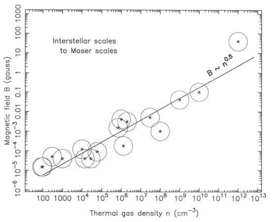 |
Figure 1. Observed behavior of the magnetic
field B (in Gauss) as a function of the
total gas density n (in cm-3), for n > 100
cm-3. The statistical results gave
B |
On the theoretical side, a 'mechanical' equilibrium model was claimed by Fleck (1988, his Table 1), who used a fragmentation order from 0 to 3, leading to B ~ n0.2 . A model with vigorous injection of turbulent energy due to expanding HII regions, stellar winds, supernovae explosions, and stellar jets was employed by Whitworth (1991) to deduce a relation Bcloud ~ 2.5 µGauss . (n / cm3)0.5 . Bhatt and Jain (1992) also predicted a B ~ 2.0 µGauss . n0.5 relation, using magnetic alignement of grains and collisional disorientation of grains, and specific grain parameters. A model of 'hierarchical' turbulences was proposed by Chaboyer and Henriksen (1990), with locally homogeneous, isotropic, and mirror symmetric turbulences, yielding a B ~ n0.6 law. A model with 2 hierarchical sequences with different types of turbulences, by Dudorov (1991), yielded a B ~ n0.5 law in one hierarchy and a B ~ n2/3 law in the other hierarchy.
Second break in behavior. At even higher gas density n,
another physical régime is
predicted. The theoretical models predict a decoupling régime
where the magnetic field
massively decouples from the cloud cores and leaves the cloud
cores, so the cloud cores own magnetic field decreases to low values
B 0 (e.g.,
Barker and Mestel 1996;
etc). The models of
Nakano and Tademaru
(1972)
and Nakano (1997)
predict that the critical gas
density for decoupling is around or above 1012
cm-3. A third break is predicted at even
higher gas density n approaching gas densities in stars, near
1024 cm-3, where we can expect
B ~ 100 Gauss due to a recoupling of B with n if
the thermal ionization of alkaline metals can
keep a high enough ionization fraction (e.g.,
Nakano 1997;
Davies 1994).
Future trends: The observational data in Table 1 just about reaches gas densities near 1011-12 cm-3. It would be interesting to observe clouds with higher gas densities and to detect or put an upper limit to B values, and thus to find the break from the B ~ n0.5 régime, i.e. the onset for the decoupling régime, as soon as more sensitive detectors come on line.