B. Redshift Surveys

1. Why do this?

Those early catalogs simply listed objects as they appeared projected onto the celestial sphere. The only indication of depth or distance came from brightness and/or size. These catalogs were, moreover, subject to human selection effects and these might vary depending on which human did the work, or even what time of the day it was.

What characterizes more recent surveys is the ability to scan photographic plates digitally (eg: the Cambridge Automatic Plate Machine, APM), or to create the survey in digital format (eg: IRAS, Sloan Survey and so on). Moreover, it is now far easier to obtain radial velocities (redshifts) for large numbers of objects in these catalogs.

Having said that, it should be noted that handling the data from these super-catalogs requires teams of dozens of astronomers doing little else. Automation of the data gathering does little to help with the data analysis!

Galaxy redshift surveys occupy a major part of the total effort and resources spent in cosmology research. Giving away hundreds of nights of telescope time for a survey, or even constructing purpose built telescopes is no light endeavour. We have to know beforehand why we are doing this, how we are going to handle and analyze the data and, most importantly, what we want to get out of it. The early work, modest as it was by comparison with the giant surveys being currently undertaken, has served to define the methods and goals for the future, and in particular have served to highlight potential problems in the data analysis.

We have come a long way from using surveys just to determine a two-point correlation function and wonder at what a fantastic straight line it is. What is probably not appreciated by those who say we have got it all wrong (eg: Sylos Labini et al. (1998)) is how much effort has gone into getting and understanding these results by a large army of people. This effort has come under intense scrutiny from other groups: that is the importance of making public the data and the techniques by which they were analyzed. The analysis of redshift data is now a highly sophisticated process leaving little room for uncertainty in the methodology: we do not simply count pairs of galaxies in some volume, normalise and plot a graph!

The prime goals of redshift surveys are to map the Universe in both physical and velocity space (particularly the deviation from uniform Hubble expansion) with a view to understanding the clustering and the dynamics. From this we can infer things about the distribution of gravitating matter and the luminosity, and we can say how they are related. This is also important when determining the global cosmological density parameters from galaxy dynamics: we are now able to measure directly the biases that arise from the fact that mass and light do not have the same distribution.

Mapping the universe in this way will provide information about how structured the Universe is now and at relatively modest redshifts. Through the cosmic microwave background radiation we have a direct view of the initial conditions that led to this structure, initial conditions that can serve as the starting point for N-body simulations. If we can put the two together we will have a pretty complete picture of our Universe and how it came to be the way it is.

Note, however, that this approach is purely experimental. We measure the properties of a large sample of galaxies, we understand the way to analyse this through N-body models, and on that basis we extract the data we want. The purist might say that there is no understanding that has grown out of this. This brings to mind the comment made by the mathematician Russell Graham in relation to computer proofs of mathematical theorems: he might ask the all-knowing computer whether the Riemann hypothesis (the last great unsolved problem of mathematics) is true. It would be immensely discouraging if the computer were to answer "Yes, it is true, but you will not be able to understand the proof". We would know that something is true without benefiting from the experience gained from proving it. This is to be compared with Andrew Wiles' proof of the Fermat Conjecture (Wiles, 1995) which was merely a corollary of some far more important issues he had discovered on his way: through proving the fundamental Taniyama-Shimura conjecture we can now relate elliptic curves and modular forms (Horgan, 1993).

We may feel the same way about running parameter-adjusted computer models of the Universe. Ultimately, we need to understand why these parameters take on the particular values assigned to them. This inevitably requires analytic or semi-analytic understanding of the underlying processes. Anything less is unsatisfactory.

2. Redshift distortions

Viewed in redshift space, which is the only three-dimensional view we have, the universe looks anisotropic: the distribution of galaxies is elongated in what have been called "fingers-of-god" pointing toward us (a phrase probably attributable to Jim Peebles). These fingers-of-god appear strongest where the galaxy density is largest (see Fig. 5), and are attributable to the extra "peculiar" (ie: non-Hubble) component of velocity in the galaxy clusters. This manifests itself as density-correlated radial noise in the radial velocity map.

Figure 5. A view of the three dimensional distribution of galaxies in which the members of the Coma cluster have been highlighted to show the characteristic "finger-of-God" pattern, from lars.

Since we know that the real 3-dimensional map should be statistically isotropic, this finger-of-god effect can be filtered out. There are several techniques for doing that: it has become particularly important in the analysis of the vast 2dF (2 degree Field) and SDSS (Sloan Digital Sky Survey) surveys (Tegmark et al., 2002). The earliest discussion of this was probably Davis and Peebles (1983).

There is another important macroscopic effect to deal with resulting from large scale flows induced by the large scale structure so clearly seen in the CfA-II Slice (de Lapparent et al., 1986). Matter is systemically flowing out of voids and into filaments; this superposes a density-dependent pattern on the redshift distribution that is not random noise as in the finger-of-god phenomenon. This distorts the map Sargent and Turner, 1977, Kaiser, 1987, Hamilton, 1998). As this distortion enhances the visual intensity of galaxy walls, which are perpendicular to the line-of-sight, it is called "the bull's-eye effect" (Praton et al., 1997).

3. Flux-limited surveys and selection functions

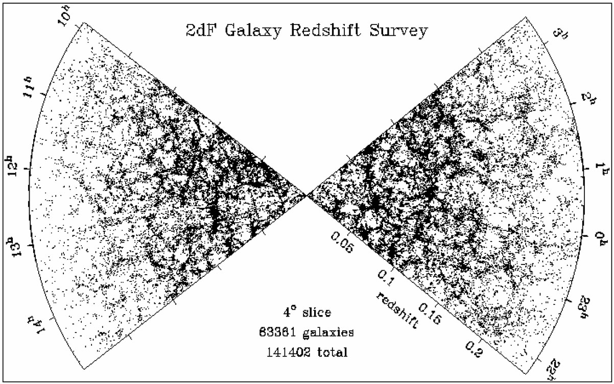
Whenever we see a cone diagram of a redshift survey (see Fig. 6), we clearly notice a gradient in the number of galaxies with redshift (or distance). This artefact is consequence of the fact that redshift surveys are flux-limited. Such surveys include all galaxies in a given region of the sky exceeding an apparent magnitude cutoff. The apparent magnitude depends logarithmically on the observed radiation flux. Thus only a small fraction of intrinsically very high luminosity galaxies are bright enough to be detected at large distances.

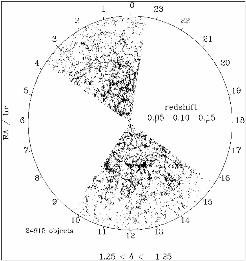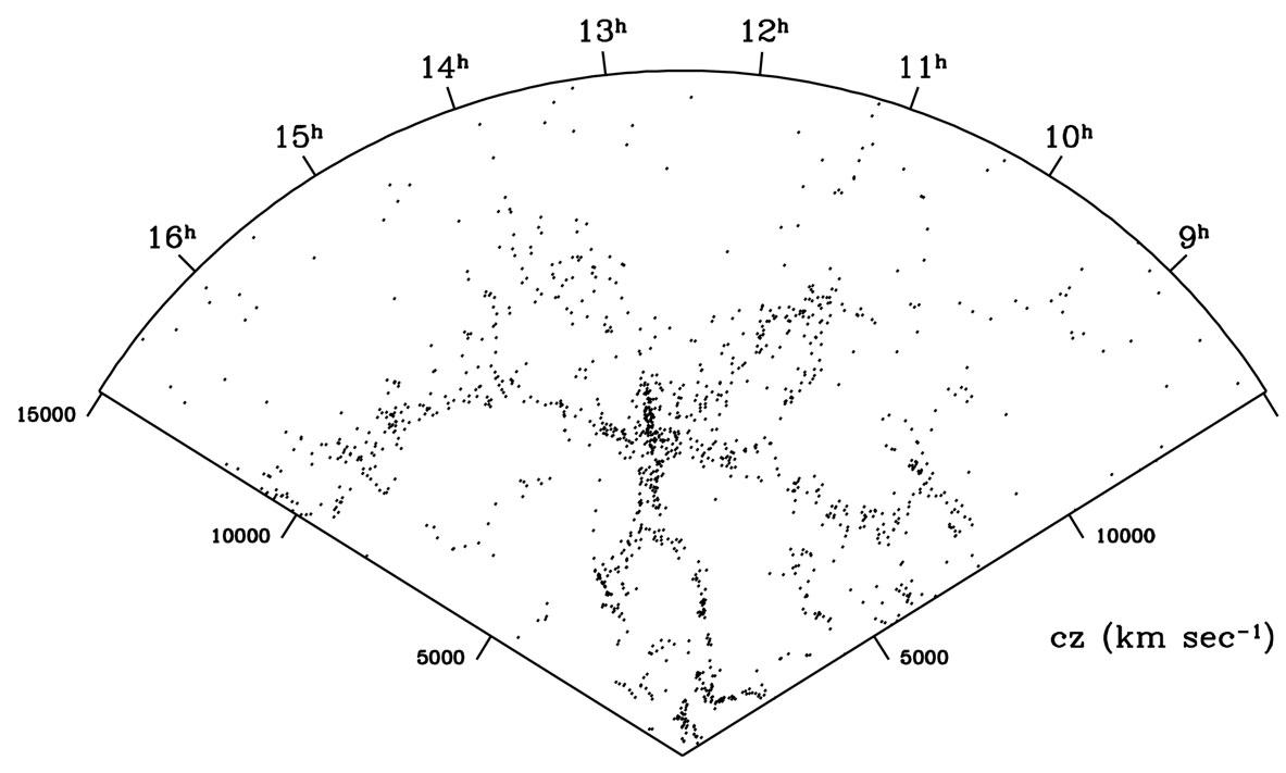
Figure 6. The top diagram shows two slices of 4° width and depth z = 0.25 from the 2dF galaxy redshift survey, from Peacock et al. (2001). The circular diagram at the bottom has a radius corresponding to redshift z = 0.2 and shows 24,915 galaxies from the SDSS survey, from (Loveday, 2002). As an inset on the right, the first CfA-II slice from de Lapparent et al. (1986) is shown to scale.

1. Extracting volume-limited samples. Given a distance limit, one can calculate, for a particular cosmological model, the minimum luminosity of a galaxy that still can be observed at that distance, considering the flux limit of the sample. Galaxies in the whole volume fainter that this luminosity will be discarded. The remaining galaxies form a homogeneous sample, but the price paid - ignoring much of the hard-earned amount of redshift information - is too high.

2. Using selection functions. For some statistical purposes, such as measuring the two-point correlation function, it is possible to use all galaxies from the flux-limited survey provided that we are able to assign a weight to each galaxy inversely proportional to the probability that a galaxy at a given distance r is included in the sample: this is dubbed the selection function (r). This quantity is usually derived from the luminosity function, which is the number density of galaxies within a given range of luminosities. A standard fit to the observed luminosity function is provided by the Schechter function (Schechter, 1976)

   (5)

   where _* is related to the total number of galaxies and the fitting parameters are L_*, a characteristic luminosity, and the scaling exponent of the power-law dominating the behavior of Eq. 5 at the faint end.

   The problem with that approach is that the luminosity function has been found to depend on local galaxy density and morphology. This is a recent discovery and has not been modelled yet.

4. Corrections to redshifts and magnitudes

The redshift distortions described earlier can be accounted for only statistically (Tegmark et al., 2002); there is no way to improve individual redshifts. However, individual measured redshifts are usually corrected for our own motion in the rest frame determined by the cosmic background radiation. This motion consists of several components (the motion of the solar system in the Galaxy, the motion of the Galaxy in the Local Group (of galaxies), and the motion of the Local Group with respect to the CMB rest frame). It is usually lumped together under the label "LG peculiar velocity" and its value is v^LG = 627 ± 22 km s^-1 toward an apex in the constellation of Hydra, with galactic latitude b = 30° ± 3° and longitude l = 276° ± 3° (see, e.g., Hamilton (1998)). If not corrected for, this velocity causes a so-called "rffect" (Kaiser, 1987), an apparent dipole density enhancement in redshift space. Application of this correction has several subtleties: see Hamilton (1998).

Most corrections to measured galaxy magnitudes are usually made during construction of a catalog, and are specific to a catalog. There is, however, one universal correction: galaxy magnitudes are obtained by measuring the flux from the galaxy in a finite width bandpass. The spectrum of a far-away galaxy is redshifted, and the flux responsible for its measured magnitude comes from different wavelengths. This correction is called the "K-correction" (Humason et al., 1956); the main problem in calculating it is insufficient knowledge of spectra of far-away (and younger) galaxies. In addition, directional corrections to magnitudes have to be considered due to the fact that the sky is not equally transparent in all directions. Part of the light coming from extragalactic objects is absorbed by the dust of the Milky Way. Due to the flat shape of our galaxy, the more obscured regions correspond to those of low galactic latitude, the so-called zone of avoidance, although the best way to account for this effect is to use the extinction maps elaborated from the observations (Schlegel et al., 1998).