3. PHYSICAL PROPERTIES AND STELLAR POPULATION

Follow-up observations of Boo were made on 25 Feb 2006 and 7 Mar 2006 (UT) with the 4m Blanco telescope at Cerro Tololo Inter-American Observatory in Chile, using the MOSAIC-II CCD camera. This comprises 8 2k × 4k pixel SITe CDDs, with a field of view 36 × 36 arcminutes and a scale of 0.27 arcseconds per pixel at the image centre. Boo was observed in the g and i bands, with exposure times of 3 × 360s in each filter on the first night and 3 × 600s in each filter on the second night, for a total exposure of 2880s in each filter. The telescope was offset ( 30 arcsecond) between exposures.

Data were processed in Cambridge using a general purpose pipeline for processing wide-field optical CCD data (Irwin & Lewis 2001). Images were de-biased and trimmed, and then flatfielded and gain-corrected to a common internal system using clipped median stacks of nightly twilight flats. The i-band images, which suffer from an additive fringing component, were also corrected using a fringe frame computed from a series of long i-band exposures taken during the night.

For each image frame, an object catalogue was generated using the object detection and parameterisation procedure discussed in Irwin et al. (2004). Astrometric calibration of the invididual frames is based on a simple Zenithal polynomical model derived from linear fits between catalogue pixel-based coordinates and standard astrometric stars derived from on-line APM plate catalogues. The astrometric solution was used to register the frames prior to creating a deep stacked image in each passband. Object catalogues were created from these stellar images and objects morphologically classified as stellar or non-stellar (or noise-like). The detected objects in each passband were merged by positional coincidence (within 1") to form a g, i combined catalogue. This catalogue was photometrically calibrated onto the SDSS system using the overlap with the SDSS catalogues.

Figure 2 shows a CMD constructed from the CTIO data. The fiducial ridgeline of the metal-poor globular cluster M92 ([Fe/H] ~ -2.3) from Clem (2005) is overplotted on the CMD. The horizontal branch is well-matched, though Boo's giant branch and MSTO are slightly blueward of the M92 isochrone. This is consistent with Boo being somewhat younger and slightly more metal-poor than M92. Note in particular the narrowness of the giant branch of the CMD in Figure 2, as evidenced by the mean color error bar shown on the left-hand side. This is characteristic of single epoch stellar populations, which are normally associated with globular clusters. However, although most dSph galaxies show evidence of multiple stellar populations, a few are known whose CMDs possess narrow red giant branches, such as Ursa Minor and Carina (van den Bergh 200b). In both cases, the narrow red giant branch is nonetheless consistent with a number of epochs of star formation (see e.g., (Shetrone et al. 2001, Koch et al. 2006.) From the fact that the horizontal branch of M92 provides a good fit, we can estimate the distance of Boo. The distance modulus is (m - M)₀ ~ 18.9 ± 0.2, corresponding to ~ 60 ± 6 kpc, where the error bar includes the uncertainty based on differences in stellar populations of Boo and M92, as well as the uncertainty in the distance of M92 . Note also that there is a prominent clump in the CMD below the horizontal branch, where Boo's blue straggler population resides.

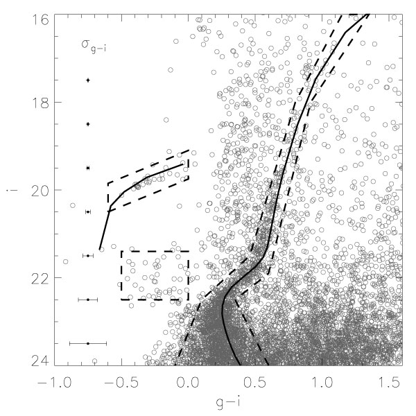Figure 2. Color-magnitude diagram of Boo derived from CTIO data. Overplotted is the ridge-line for the old, metal-poor globular cluster M92. The dashed lines are used to select stars belonging to the main sequence, giant branch and horizontal branch of the satellite. For each magnitude bin, the mean color error is shown on the left-hand side.

Even though the CMD resembles that of a globular cluster, this is emphatically not the case for the object's morphology and size. To select candidate stars, we use the boundaries marked by the dashed lines on the CMD, which wrap around the satellite sequence. SDSS data are used here as the CTIO data are largely confined to the inner parts of Boo. The locations of SDSS stars with r < 23 lying within the boundaries are plotted in the top panel of Fig. 3. These objects are binned into 30 × 30 bins, each 0.033° × 0.033°, and smoothed with a Gaussian with FWHM of 0.067° to yield the plot in the lower panel. The density contours, representing 1.5, 3, 5, 7, 10 and 13 above the background level, are elongated and irregular - more so than even the most irregular of the Galactic dSphs, Ursa Minor (see e.g., Palma et al. 2003). The black dots are candidate blue horizontal branch stars and open circles are blue stragglers. The spatial distribution of both populations is roughly consistent with the underlying density contours and shows the same tail-like extensions. There are hints that Boo could be a much larger object, as the blue horizontal branch and straggler population extend beyond the outermost contours.

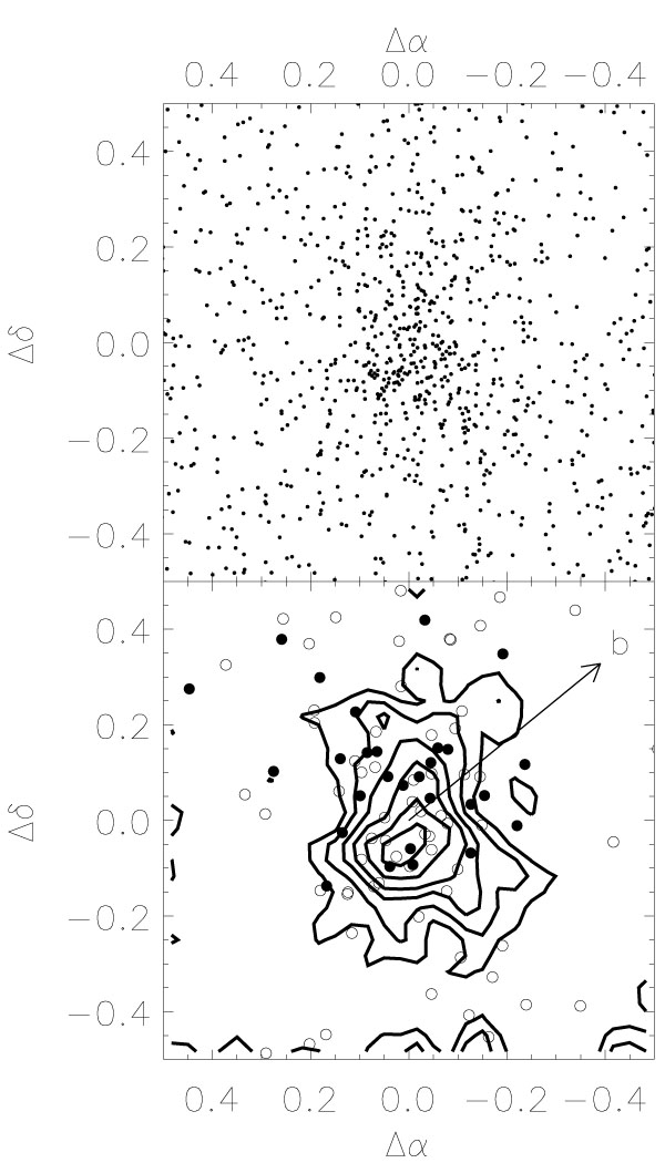Figure 3. Morphology of Boo: Upper: The spatial distribution of SDSS stars selected from CMD regions marked with dashed lines in Fig. 1. Lower: A contour plot of the spatial distribution of Boo's stars; candidate blue horizontal branch stars and blue stragglers (from the boxes in the CMD) are overplotted with black dots and open circles. The contours are 1.5, 3, 5, 7, 10 and 13 above the background level. The direction of increasing Galactic latitude is marked by an arrow.

To estimate the properties listed in Table 1, we use the SDSS data shown in Figure 3 to derive the centroid from the density-weighted first moment of the distribution, and the average ellipticity and position angle using the three density-weighted second moments (e.g. Stobie 1980). The radial profile shown in Figure 4 is derived by computing the average density within elliptical annuli after first subtracting a constant asymptotic background level (0.2 arcminute^-2) reached at large radii. We then fit the radial profile with standard Plummer and exponential laws (Figure 4, see also Irwin & Hatzidimitriou 1995). The best-fitting position angle, ellipticity and half-light radius are listed in Table 1. At a distance of ~ 60 kpc, the half-light radius of 130 corresponds to ~ 220 pc. This is the typical scale length of the Galactic dSph galaxies, and a factor of ~ 10 times larger than the scale length of the largest Galactic globular clusters. Note that neither the Plummer nor the exponential laws provide exceptional fits to the data - in particular, the center of the object is not well-fitted and appears to lack a clearly defined core. Although Boo appears superficially somewhat similar to Willman 1, it is substantially larger and more luminous. Willman 1 has a characteristic scale length of only ~ 20 pc and an absolute magnitude of M_tot,V ~ -2^m.5. The stellar populations are also different - for example, Willman 1 has no red giant or horizontal branch stars (Willman et al. 2006).

Table 1. Properties of the Boötes Satellite

Parameter a
Coordinates (J2000)	14:00:06   +14:30:00 ± 15
Coordinates (Galactic)	= 358.1°, b = 69.6°
Position Angle	10° ± 10°
Ellipticity	0.33
rh(Plummer)	13.'0 ± 0.'7
rh(Exponential)	12.'6 ± 0.'7
AV	0m.06
µ0,V(Plummer)	28m.3 ± 0m.5
µ0,V(Exponential)	27m.8 ± 0m.5
Vtot	13m.6 ± 0m.5
(m-M)0	18m.9 ± 0m.20
Mtot,V	-5m.8 ± 0m.5
a Surface brightnesses and integrated magnitudes are corrected for the mean Galactic foreground reddenings, AV, shown.

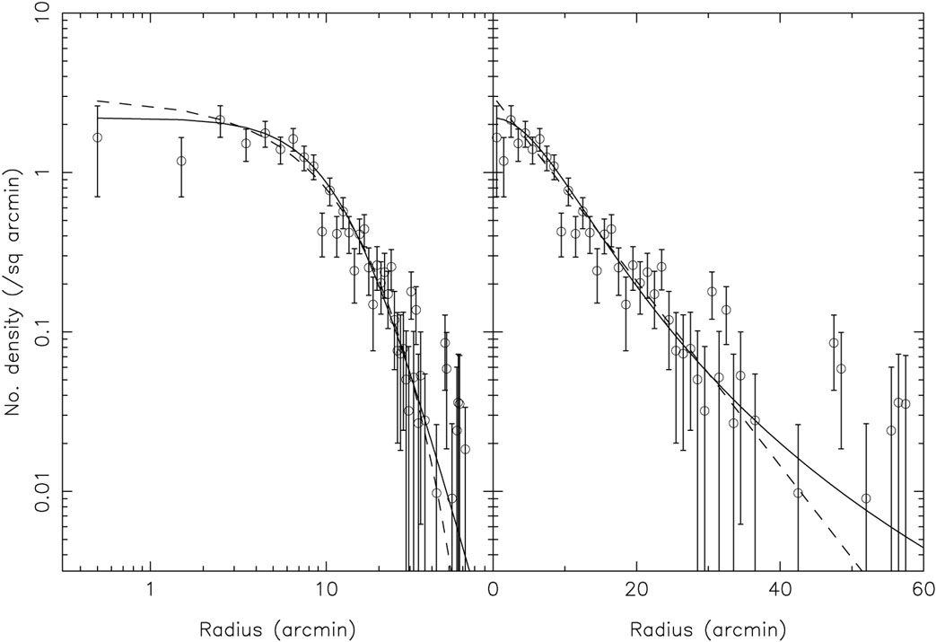Figure 4. Profile of Boo, showing the stellar density in elliptical annuli as a function of mean radius. The left panel is logarithmic in both axes, and the right panel is linear in radius. The overplotted lines are fitted Plummer (solid) and exponential (dashed) profiles.

The overall luminosity is computed by masking the stellar locus of Boo in the CMD in Figure 1 and computing the total flux within the mask and within the elliptical half-light radius. A similar mask, but covering a larger area to minimize shot-noise, well outside the main body of Boo is scaled by relative area and used to compute the foreground contamination within the half-light radius. After correcting for this contamination, the remaining flux is scaled to the total, assuming the fitted profiles are a fair representation of the overall flux distribution. We also apply a correction of 0.3 magnitudes for unresolved/faint stars, based on the stellar luminosity functions of other low metallicity, low surface brightness dSphs. The resulting luminosity estimate is M_tot,V ~ -5^m.8. Applying our procedure to the Ursa Major dSph, discovered by Willman et al. (2005), gives M_tot,V ~ -5^m.5. We conclude that Boo is, within the uncertainties, comparable in faintness to Ursa Major.

We argue that Boo is not a tidally disrupted globular cluster as follows. First, it is much too extended. If a globular cluster is tidally disrupted, its half-light radius may increase somewhat, but it does not grow to such an immense radius as ~ 220 pc. Second, for it to be a destroyed globular cluster, Boo would have to be on a plunging radial orbit. Then the outermost isodensity contours, which should be aligned with the direction of the proper motion, should point towards the Galactic center. This is not the case, as judged from Fig. 3. Third, globular clusters often show evidence for mass segregation driven by internal dynamical evolution (see e.g. Koch et al. 2004). Accordingly, Figure 5 shows normalized luminosity functions (LFs) for the inner and outer parts of Boo constructed with the CTIO data. There is no evidence for substantial mass segregation in Boo with the present data. However, this data are largely restricted to stars of similar mass, and deeper data are required to give a conclusive result.

Figure 5. Normalized luminosity functions of the inner (solid) and outer (dashed) parts of Boo, constructed with the CTIO data. The main sequence turn-off is indicated by the arrow.