3. HARD X-RAY EMISSION

The two possibilities here are Bremsstrahlung (thermal or non-thermal) emission by a nonrelativistic electron population and IC emission by extreme relativistic electrons which are also responsible for the observed radio emission. There are difficulties in both cases but as we show below the IC is the most likely interpretation. Fig. 2 gives the timescales for the relevant processes for typical ICM conditions.

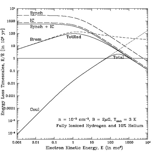Figure 2. Radiative, cold target Coulomb collision loss and other relevant timescales as a function of energy for the specified ICM conditions. The solid lines from top to bottom give the IC plus synchrotron, total radiative and total loss timescales. From Petrosian (2001).

3.1. Bremsstrahlung emission

Bremsstrahlung radiation in the HXR (20 to 100 keV) range requires electrons of comparable or somewhat larger energies. As pointed out by Petrosian (2001, P01 for short), and as evident from Fig. 2, for such nonrelativisitic electrons NT Bremsstrahlung losses are negligible compared to elastic Coulomb losses. A thermal Bremsstrahlung interpretation of this emission requires temperatures well above the virial value (see also below). Very generally, for a particle of energy E interacting with background electrons and protons of much lower energy (cold target), the energy yield in Bremsstrahlung photons Y_{brem brem} / _Coul = (4 ln / 3)(E / m_e c²) ~ 3 × 10^-6(E / 25 keV). Here is the fine structure constant and ln , the Coulomb logarithm, is ~ 40 for ICM conditions (for details see Petrosian 1973). Note that this result is independent of the spectrum of emitting electrons which could be a Maxwellian of higher temperature (T_hot ~ 30 keV) or a power law of mean energy >> kT of the background particles ¹. As pointed out in P01, for continuous production of a HXR luminosity of L_HXR(~ 4 × 10⁴³ erg s^-1 estimated for Coma, see Table 1), a power of L_HXR / Y_brem(~ 10⁴⁹ erg s^-1 for Coma) must be continuously fed into the ICM. This will increase the ICM temperature to T ~ 10⁸ K after 6 × 10⁷ yr, or to 10¹⁰ K in a Hubble time. An obvious conclusion here is that the HXR Bremsstrahlung emission phase must be very short lived. It should also be noted that such a hot gas or such high energy electrons cannot be confined in the ICM by gravity and will escape it in a crossing time of ~ 3 × 10⁶ yr unless it is confined by the magnetic field or by scattering. From Fig. 2 we see that the Coulomb scattering time, which is comparable to the Coulomb loss time, is equal to the crossing time so that the escape time of the particles will be comparable to these. Therefore, for confinement for periods exceeding the loss time we need a shorter scattering mean free path or timescale. For example, for the scattering timescale shown in this figure the escape time will be larger than the total electron loss time at all energies.

These estimates of short timescales are based on energy losses of electrons in a cold plasma which is an excellent approximation for electron energies E >> kT (or for T_hot >> T). As E nears kT the Coulomb energy loss rate increases and the Bremsstrahlung yield decreases. For E / kT > 4 we estimate that this increase will be at most about a factor of 3 (see below).

An exact treatment of the particle spectra in the energy regime close to the thermal pool requires a solution of non-linear kinetic equations instead of the quasi-linear approach justified for high energy particles where they can be considered as test particles. Apart from Coulomb collisions, also collisionless relaxation processes could play a role in the shaping of supra-thermal particle spectra (i.e. in the energy regime just above the particle kinetic temperature). We have illustrated the effect of fast collisionless relaxation of ions in a post-shock flow in Figs. 1 and 2 of Bykov et al. 2008 - Chapter 8, this volume. The relaxation problem has some common features with N-body simulations of cluster virialisation discussed in other papers of this volume where collisionless relaxation effects are important. The appropriate kinetic equations to describe both of the effects are non-linear integro-differential equations and thus by now some simplified approximation schemes were used.

In a recent paper Dogiel et al. (2007) using linear Fokker-Planck equations for test particles concluded that in spite of the short lifetime of the test particles the "particle distribution" lifetime is longer and a power law tail can be maintained by stochastic turbulent acceleration without requiring the energy input estimated above. In what follows we address this problem not with the test particles and cold plasma assumption, but by carrying out a calculation of lifetimes of NT high energy tails in the ICM plasma. The proposed approach is based on still linearised, but more realistic kinetic equations for Coulomb relaxation of an initial distribution of NT particles.

3.1.1. Hot plasma loss times and thermalisation

The energy loss rate or relaxation into a thermal distribution of high energy electrons in a magnetised plasma can be treated by the Fokker-Planck transport equation for the gyro-phased average distribution along the length s of the field lines F(t, E, µ, s), where µ stands for the pitch angle cosine. Assuming an isotropic pitch angle distribution and a homogeneous source (or more realistically integrating over the whole volume of the region) the transport equation describing the pitch angle averaged spectrum, N(E, t) F ds dµ, of the particles can be written as (see Petrosian & Bykov 2008 - Chapter 11, this volume for more details):

(1)

where D_Coul(E) and _Coul(E) describe the energy diffusion coefficient and energy loss (+) or gain (-) rate due to Coulomb collisions. We have ignored Bremsstrahlung and IC and synchrotron losses, which are negligible compared to Coulomb losses at low energies and for typical ICM conditions.

As mentioned above, the previous analysis was based on an energy loss rate due to Coulomb collisions with a "cold" ambient plasma (target electrons having zero velocity):

(2)

v = c is the particle velocity and r₀ = e² / (m_e c² ) = 2.8 × 10^-13 cm is the classical electron radius. For ICM density of n = 10^-3 cm^-3, and a Coulomb logarithm ln = 40, _Coul = 2.7 × 10⁷ yr. Note that the diffusion coefficient is zero for a cold target so that N / t = _Coul^-1 / E [N / ] from which one can readily get the results summarised above. As stated above this form of the loss rate is a good approximation when the NT electron velocity v >> v_th, where v_th = (2kT / m_e)^1/2 is the thermal velocity of the background electrons. This approximation becomes worse as v v_th and breaks down completely for v < v_th, in which case the electron may gain energy rather than lose energy as is always the case in the cold-target scenario. A more general treatment of Coulomb loss is therefore desired. Petrosian & East (2007, PE07 herafter) describe such a treatment. We summarise their results below. For details the reader is referred to that paper and the references cited therein.

Let us first consider the energy loss rate. This is obtained from the rate of exchange of energy between two electrons with energies E and E' which we write as

(3)

Here G(E, E') is an antisymmetric function of the two variables such that the higher energy electrons loses and the lower one gains energy (see e.g. Nayakshin & Melia 1998). From their Eq. 24-26 we can write

(4)

The general Coulomb loss term is obtained by integrating over the particle distribution:

(5)

For non-relativistic particles this reduces to

(6)

Similarly, the Coulomb diffusion coefficient can be obtained from

(7)

as D_Coul^gen(E, t) = (m_e² c⁴ / _Coul) ₀ H(E, E')N(E', t)dE'. From equations (35) and (36) of Nayakshin & Melia (1998) ² we get

(8)

Again, for nonrelativistic energies the Coulomb diffusion coefficient becomes

(9)

Thus, the determination of the distribution N(E, t) involves solution of the combined integro-differential equations Eq. 1, 6 and 9, which can be solved iteratively. However, in many cases these equations can be simplified considerably. For example, if the bulk of the particles have a Maxwellian distribution

(10)

with kT << m_e c², then integrating over this energy distribution, and after some algebra, the net energy loss (gain) rate and the diffusion coefficient can be written as (see references in PE07):

(11)

and

(12)

where erf(x) = 2 / ^1/2 ₀^x e^-t2 dt is the error function.

The numerical results presented below are based on another commonly used form of the transport equation in the code developed by Park & Petrosian (1995, 1996), where the diffusion term in Eq. 1 is written as / E [D(E) / E N(E)]. This requires modification of the loss term to

(13)

where we have used Eqs. 11 and 12. Fig. 3 shows the loss and diffusion times,

(14)

and

(15)

based on the above equations.

Figure 3. Various timescales for Coulomb collisions for hot and cold plasma with typical ICM parameters from Eqs. 2, 11, 12 and 13. Note that the as we approach the energy E kT the loss time increases and eventually becomes negative (or gain time) at low energies. The portions below the spike show the absolute value of these timescales. From Petrosian & East (2007).

As a test of this algorithm PE07 show that an initially narrow distribution of particles (say, Gaussian with mean energy E₀ and width E << E₀) subject only to Coulomb collisions approaches a Maxwellian with kT = 2E₀ / 3 with a constant total number of particles within several times the theoretically expected thermalisation time, which is related to our _Coul as (see Spitzer 1962 or Benz 2002)

(16)

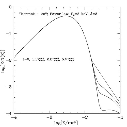
Using the above equations one can determine the thermalisation or the energy loss timescale of supra-thermal tails into a background thermal distribution. Fig. 4 shows two examples of the evolution of an injected power-law distribution of electrons. The left panel shows this evolution assuming a constant temperature background plasma, which would be the case if either the energy of the injected electrons was negligible compared to that of the background electrons, or if the energy lost by the injected particles is lost by some other means. The right panel does not make these assumptions and allows the whole distribution to evolve. As is clearly seen in this figure, the energy lost by the NT particles heats the plasma. It is also evident that the NT tail is peeled away starting with low energies and progressing to higher ones. The NT tail becomes negligible within less than 100 times the thermalisation time of the background particles. These times are only about three times larger than the timescale one gets based on a cold target assumption for E₀ = 20 keV particles. Similar conclusions were reached by Wolfe & Melia (2006). The change in the electron lifetime agrees also with Fig. 3 of Dogiel et al. (2007). But our results do not support the other claims in their paper about the longer lifetime of the "distribution of particles". The results presented here also seem to disagree with Blasi (2000), where a procedure very similar to ours was used (for more details see PE07).

Figure 4. Evolution of a NT power law tail (with isotropic angular distribution) of electrons subject to elastic Coulomb collisions with background thermal plasma electrons with initial temperature kT = 1 keV, showing gradual degradation of the power law NT tail (starting at energy E0 with spectral index ). Left panel: Here we assume that the energy input by the NT tail is negligible or carried away by some other means; i.e. the temperature of the plasma is forced to remain constant. Right panel: Here the energy of the NT particles remains in the system so that their thermalisation heats the plasma. In both cases the NT tails are reduced by a factor of ten within less than 100 × therm or < 3 times the cold target loss time at the injected energy. From Petrosian & East (2007).

3.2. Emission from relativistic electrons

The radiative efficiency of relativistic electrons is much higher than that of nonrelativisitic ones because of lower Coulomb losses (see Fig. 2). For ICM conditions electrons with GeV or higher energies lose energy via synchrotron and IC mechanisms. At such energies the Bremsstrahlung rate receives contributions from both electron-electron and electron-ion interactions and its loss rate becomes larger than Coulomb rate but remains below IC and synchrotron rates. Nevertheless, Bremsstrahlung emission could be the main source of gamma-ray radiation in the GLAST range (> GeV). In this section we first compare the first two processes and explore whether the same population of electrons can be responsible for both radio and HXR emissions. Then we consider Bremsstrahlung and other processes for the gamma-ray range.

3.2.1. Hard X-ray and radio emission

As stated in the introduction, relativistic electrons of similar energies ( > 10³) can be responsible for both the IC-HXR and synchrotron-radio emission. The IC and synchrotron fluxes depend on the photon (CMB in our case) and magnetic field energy densities and their spectra depend on the spectrum of the electrons (see e.g. Rybicki & Lightman 1979). For a power law distribution of relativistic electrons, N () = N_total(p - 1) ^-p _min^p-1, and for > _min, the spectrum of both radiation components, from a source at redshift z Z - 1 and co-moving coordinate r(Z), is given by

(17)

where d_L(Z) = (c / H₀)Zr(Z) is the luminosity distance and = (p + 1) / 2 is the photon number spectral index ³. This also assumes that the relativistic electrons and the magnetic field have similar spatial distribution so that the spatial distribution of HXRs and radio emission are the same (see e.g. Rephaeli 1979). The clusters are unresolved at HXRs so at this time this is the most reasonable and simplest assumption. A larger HXR flux will be the result if the electron and B field distributions are widely separated (see e.g., Brunetti et al. 2001).

For synchrotron _{cr, synch} = 3_min² _B / 2, with _B = e B / (2 m_e c) and u_synch = B² / (8), and for IC, u_i is the soft photon energy density and _cr,IC = _min² < h >. For black body photons u_IC = (8⁵ / 15)(kT)⁴ / (hc)³ and < h > = 2.8 kT. A_i are some simple functions of the electron index p and are of the order of unity and are given in Rybicki & Lightman (1979). Given the cluster redshift we know the temperature of the CMB photons (T = T₀ Z) and that _cr,IC Z and u_IC Z⁴ so that we have

(18)

Consequently, from the observed ratio of fluxes we can determine the strength of the magnetic field.

For Coma, this requires the volume averaged magnetic field to be ~ 0.1 µG, while equipartition gives ~ 0.4 µG and Faraday rotation measurements give the average line of sight field of _l ~ 3 µG (Giovannini et al. 1993, Kim et al. 1990, Clarke et al. 2001, Clarke 2003). In general the Faraday rotation measurements of most clusters give B > 1 µG; see e.g. Govoni et al. 2003. However, there are several factors which may resolve this discrepancy. Firstly, the last value assumes a chaotic magnetic field with a scale of a few kpc which is not a directly measured quantity (see e.g., Carilli & Taylor 2002) ⁴. Secondly, the accuracy of these results has been questioned (Rudnick & Blundell 2003; but see Govoni & Feretti 2004 for an opposing point of view). Thirdly, as shown by Goldshmidt & Rephaeli (1993), and also pointed out by Brunetti et al. (2001), a strong gradient in the magnetic field can reconcile the difference between the volume and line-of-sight averaged measurements. Finally, as pointed out by P01, this discrepancy can be alleviated by a more realistic electron spectral distribution (e.g. the spectrum with exponential cutoff suggested by Schlickeiser et al. (1987) and/or a non-isotropic pitch angle distribution). In addition, for a population of clusters observational selection effects come into play and may favour Faraday rotation detection in high B clusters which will have a weaker IC flux relative to synchrotron. The above discussion indicates that the Faraday rotation measurements are somewhat controversial and do not provide a solid evidence against the IC model.

We now give some of the details relating the various observables in the IC model. We assume some proportional relation (e.g. equipartition) between the energies of the magnetic field and non-thermal electrons

(19)

where R = d_A / 2 is the radius of the (assumed) spherical cluster with measured angular diameter and angular diameter distance d_A(Z) = (c / H₀)r(Z) / Z, and equipartition with electrons is equivalent to = 1.

From the three equations (17), (18) and (19) we can determine the three unknowns B, _e (or N_total) and F_HXR purely in terms of , _min, and the observed quantities (given in Table 1) z, and the radio flux F_radio(). The result is ⁵

(20)

(21)

and

(22)

where we have defined F₀ 10^-11 erg cm^-2 s^-1. Note also that in all these expressions one may use the radius of the cluster R = 3.39 Mpc ( / 5') r(Z) / Z instead of the angular radius .

Table 1. Observed and estimated properties of clusters

Cluster	z	kT a	F1.4 GHz b	c,b	FSXR	Bd	FHXR e
		(keV)	(mJy)	(arcmin)	(F0) f	(µG)	(F0) f
Coma	0.023	7.9	52	30	33	0.40	1.4 (1.6)
A 2256	0.058	7.5	400	12	5.1	1.1	1.8 (1.0)
1ES 0657-55.8	0.296	15.6	78	5	3.9	1.2	0.52 (0.5)
A 2219	0.226	12.4	81	8	2.4	0.86	1.0
A 2163	0.208	13.8	55	6	3.3	0.97	0.50 (1.1)
MCS J0717.5+3745	0.550	13	220	3	3.5	2.6	0.76
A 1914	0.171	10.7	50	4	1.8	1.3	0.22
A 2744	0.308	11.0	38	5	0.76	1.0	0.41
a From Allen & Fabian (1998), except 1ES 0657-55.8 data from Liang et al. (2000) b Data for Coma from Kim et al. (1990); A 2256, A 2163, A 1914 and A 2744 from Giovannini et al. (1999); 1ES 0657-55.8 from Liang et al. (2000); A 2219 from Bacchi et al. (2003). c Approximate largest angular extent. d Estimates based on equipartition. e Estimates assuming min = 106, with observed values in parentheses: Coma (Rephaeli et al. 1999, Rephaeli & Gruber 2002, Fusco-Femiano et al. 1999, Fusco-Femiano et al. 2003); Abell 2256 (Fusco-Femiano et al. 2000, Fusco-Femiano et al. 2004, Rephaeli & Gruber 2003); 1ES 0657-55.8 (Petrosian et al. 2006); Abell 2163 (Rephaeli et al. 2006) these last authors also give a volume averaged B ~ 0.4 ± 0.2 µG. f F0 10-11 erg cm-2 s-1

Table 1 presents a list of clusters with observed HXR emission and some other promising candidates. To obtain numerical estimates of the above quantities in addition to the observables F_radio, and redshift z we need the values of and _min. Very little is known about these two parameters and how they may vary from cluster to cluster. From the radio observations at the lowest frequency we can set an upper limit on _min; for Coma e.g., assuming B ~ µG we get _min < 4 × 10³ (µG / B). We also know that the cut off energy cannot be too low because for p > 3 most of the energy of electrons (_e = _min ² N() d) resides in the low energy end of the spectrum. As evident from Fig. 2 electrons with < 100 will lose their energy primarily via Coulomb collisions and heat the ICM. Thus, extending the spectra below this energy will cause excessive heating. A conservative estimate will be _min ~ 10³. Even less is known about . The estimated values of the magnetic fields B for the simple case of = 2, equipartition (i.e. = 1) and low energy cut off _min = 10³ are given in the 7th column of Table 1. As expected these are of the order of a few µG; for significantly stronger field, the predicted HXR fluxes will be below what is detected (or even potentially detectable). For = 2 the magnetic field B ( _min)^-1/4 and F_HXR ( _min)^1/2 so that for sub-µG fields and F_HXR ~ F₀ we need _min ~ 10⁶. Assuming _min = 10³ and = 10³ we have calculated the expected fluxes integrated in the range of 20-100 keV (which for = 2 is equal to 1.62 × [20 keV F_HXR(20 keV)]), shown on the last column of Table 1. The variation of this flux with redshift based on the observed parameters, and F_radio( = 1.4 GHz) of Coma and A 2256 are plotted in Fig. 5 for three values of = 1.75, 2.0 and 2.25 (p = 2.5, 3 and 3.5) and assuming a constant physical radius R which is a reasonable assumption. We also plot the same assuming a constant angular diameter. This could be the case due to observational selection bias if diffuse radio emission is seen mainly from sources with near the resolution of the telescopes. These are clearly uncertain procedures and can give only semi-quantitative measures. However, the fact that the few observed values (given in parenthesis) are close to the predicted values is encouraging.

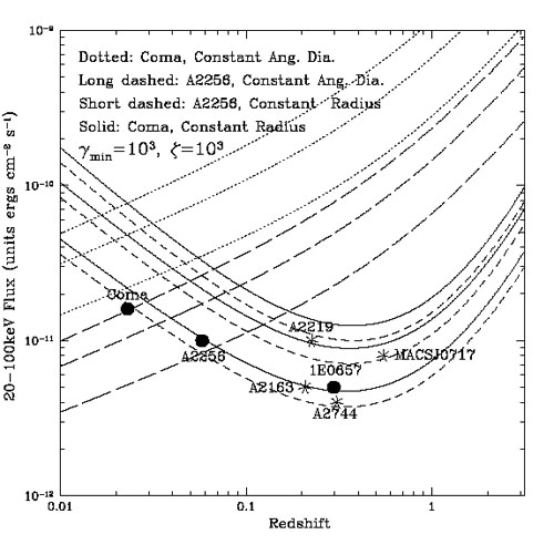Figure 5. Predicted variations of the HXR flux with redshift assuming a constant physical diameter (solid and dashed lines) or constant angular diameter (dotted and long-dashed lines), using the Coma cluster (dotted and solid) and A 2256 (long or short dashed) parameters assuming = min = 103. In each group, the IC photon spectral index = 2.25, 2.0, 1.75, from top to bottom. Filled circles are based on observations and stars based on the estimates given in Table 1. From Petrosian et al. (2006).

Our estimates indicate that ~ 10⁶ / _min > 10³. In addition to the caveats enumerated above we note that, as described by Petrosian & Bykov 2008 - Chapter 11, this volume, the sources generating the magnetic fields and the high energy electrons may not be identical so that equipartition might not be what one would expect.

The spectrum of the required high energy electrons is best constrained by the radio observations. In Fig. 1 we showed two possible synchrotron spectra. The corresponding electron spectra are shown in Fig. 6 along with the Maxwellian distribution of thermal electrons. The low end of the NT spectra are constrained by requiring that their Coulomb loss rate be small so that there will not be an excessive heating of the background particles. These span the kind of NT electron spectrum that the acceleration model, discussed by Petrosian & Bykov 2008 - Chapter 11, this volume, must produce.

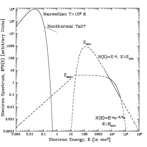Figure 6. The spectrum of electrons required for production of radio and HXR radiation based on the synchrotron and IC models. Values representing the Coma cluster are used. The low energy peak shows the distribution of thermal electrons along with a NT tail that would be required if the HXRs are produced by the non-thermal Bremsstrahlung mechanism. The low end of the high energy NT electrons are constrained to avoid excessive heating. The corresponding radio synchrotron spectra are shown in Fig. 1. From Petrosian (2003).

3.2.2. Gamma-ray emission

There have been several estimates of the expected gamma-ray flux, specifically from Coma (see e.g. Atoyan & Völk 2000, Bykov et al. 2000, Reimer et al. 2004, Blasi et al. 2007). The EGRET upper limit shown in Fig. 1 does not provide stringent constraints but GLAST with its much higher sensitivity can shed light on the processes described above. Several processes can produce gamma-ray radiation. Among electronic processes one expects IC and Bremsstrahlung radiation if electrons have sufficiently high energies. If the electron spectrum that accounts for radio and HXR emission can be extended to Lorentz factors of 3 × 10⁵ (say with spectral index p = 3-4) then the IC scattering of CMB photons can produce 100 MeV radiation with a F() flux comparable to the HXR fluxes (~ 10^-11 - 10^-12 erg cm^-2 s^-1) which can easily be detected by GLAST (the former actually disagrees with the EGRET upper limit shown in Fig. 1). The lifetime of such electrons is less than 10⁷ years so that whatever the mechanism of their production (injection from galaxies or AGN, secondary electrons from proton-proton interactions, see the discussion by Petrosian & Bykov 2008 - Chapter 11, this volume), these electrons must be produced throughout the cluster within times shorter than their lifetime. A second source could be electrons with > 10⁴ scattering against the far infrared background (or cosmic background light) which will produce > 10 MeV photons but with a flux which is more than 100 times lower than the HXR flux (assuming a cosmic background light to CMB energy density ratio of < 10^-2) which would be comparable to the GLAST one year threshold of ~ 10^-13 erg cm^-2 s^-1. IC scattering of more abundant SXR photons by these electrons could produce > 100 MeV gamma-rays but the rate is suppressed by the Klein-Nishina effect. Only lower energy electrons < 10² will not suffer from this effect and could give rise to 100 MeV photons. As shown in Fig. 6 this is the lowest energy that a p = 3 spectrum can be extended to without causing excessive heating (see P01). These also may be the most abundant electrons because they have the longest lifetime (see Fig. 2). The expected gamma-ray flux will be greater than the GLAST threshold.

High energy electrons can also produce NT Bremsstrahlung photons with energies somewhat smaller than their energy. Thus, radio and HXR producing electrons will produce greater than 1 GeV photons. Because for each process the radiative loss rate roughly scales as = E / _loss, the ratio of the of gamma-ray to HXR fluxes will be comparable to the inverse of the loss times of Bremsstrahlung _brem and IC _IC shown in Fig. 2 (~ 10^-2 for ~ 10⁴), which is just above the GLAST threshold.

Finally hadronic processes by cosmic rays (mainly p - p scattering) can give rise to ~ 100 MeV and greater gamma-rays from the decay of ⁰ produced in these scatterings. The ^± decays give the secondary electrons which can contribute to the above radiation mechanisms. This is an attractive scenario because for cosmic ray protons the loss time is long and given an appropriate scattering agent, they can be confined in the ICM for a Hubble time (see, Berezinsky et al. 1997 and the discussion by Petrosian & Bykov 2008 - Chapter 11, this volume). It is difficult to estimate the fluxes of this radiation because at the present time there are no observational constraints on the density of cosmic ray protons in the ICM. There is theoretical speculation that their energy density may be comparable to that of the thermal gas in which case the gamma-ray flux can be easily detected by GLAST. Reimer et al. (2004) estimate that GLAST can detect gamma-rays from the decay of ⁰'s if the cosmic ray proton energy is about 10% of the cluster thermal energy.

¹ As shown below, also from the acceleration point of view for this scenario, the thermal and NT cases cannot be easily distinguished from each other. The acceleration mechanism energises the plasma and modifies its distribution in a way that both heating and acceleration take place. Back.

² Note that the first term in their equation (35) should have a minus sign and that the whole quantity is too large by a factor of 2; see also Blasi (2000) for other typos. Back.

³ These expressions are valid for spectral index p > 3 or > 2. For smaller indices an upper energy limit _max must also be specified and the above expressions must be modified by other factors which are omitted here for the sake of simplification. Back.

⁴ The average line of sight component of the magnetic field in a chaotic field of scale _chaos will be roughly _chaos / R times the mean value of the magnetic field, where R is the size of the region. Back.

⁵ Here we have set the Hubble constant H₀ = 70 km s^-1 Mpc^-1, the CMB temperature T₀ = 2.8 K, and the radio frequency = 1.4 GHz. In general B²⁺ H₀ ^-1, N_total H₀^-3 and F_HXR H₀² T₀²⁺. We have also assumed an isotropic distribution of the electron pitch angles and set B = B(4 / ). Back.