Copyright © 2004 by Annual Reviews. All rights reserved
| Annu. Rev. Astron. Astrophys. 2004. 42:
211-273 Copyright © 2004 by Annual Reviews. All rights reserved |


The interstellar medium presents a bewildering variety of intricate structures and complex motions that cannot be compressed entirely into a few numbers or functions (Figures 1 and 2). Any identification with physical processes or simulations must involve a large set of diagnostic tools. Here we begin with analysis techniques involving correlation functions, structure functions, and other statistical descriptors of column density and brightness temperature, and then we discuss techniques that include velocities and emission-line profiles.
 |
Figure 1. CO emission from the outer Galaxy spanning a range of Galactic longitude from 102.5° to 141.5° and latitude from -3° to 5.4°, sampled every 50" with a 45" beam. The emission is integrated between -110 km s-1 and 20 km s-1. The high latitude emission is mostly from local gas at low velocity, consisting of small structures that tend to be nonself-gravitating. The low latitude emission is a combination of local gas plus gas in the Perseus arm at higher velocity. The Perseus arm gas includes the giant self-gravitating clouds that formed the OB associations that excite W3, W4, and W5 (left) and NGC 7538 (right). Most structures are hierarchical and self-similar on different scales, so the distant massive clouds look about the same on this map as the local low-mass clouds. This image was kindly provided by M. Heyer using data from Heyer et al. (1998). |
 |
Figure 2. Integrated H I emission from the LMC showing shells and filaments covering a wide range of scales. The 2D power spectrum of this emission is a power law from 20 pc to 1 kpc with a slope of ~ -3.2. Data from Elmegreen, Kim & Staveley-Smith (2001). |
Interstellar turbulence has been characterized by structure functions, autocorrelations, power spectra, energy spectra, and delta variance, all of which are based on the same basic operation. The structure function of order p for an observable A is
 |
(1) |
for position r and increment
 r, and the
power-law fit to this,
Sp(r)
r, and the
power-law fit to this,
Sp(r)
 r
r p, gives the
slope p.
The autocorrelation of A is
p, gives the
slope p.
The autocorrelation of A is
 |
(2) |
and the power spectrum is
 |
(3) |
for Fourier transform  =
=
 eikr A(r)dr and complex
conjugate A*. The Delta variance
(Stützki et
al. 1998,
Zielinsky &
Stützki 1999)
is a way to measure power on various scales using an unsharp mask:
eikr A(r)dr and complex
conjugate A*. The Delta variance
(Stützki et
al. 1998,
Zielinsky &
Stützki 1999)
is a way to measure power on various scales using an unsharp mask:
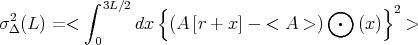 |
(4) |
for a two-step function
 |
(5) |
In these equations, the average over the map, indicated by <>, is used as an estimate of the ensemble average.
The power spectrum is the Fourier transform of the autocorrelation
function, and for a statistically homogeneous and isotropic field,
the structure function-of-order p = 2 is the mean-squared A
minus twice the autocorrelation: S2 =
<A2> - 2C. The delta
variance is related to the power spectrum: For an emission
distribution with a power spectrum
k-n for wave number k, the delta variance is
rn-2 for r = 1 / k
(Bensch, Stützki
& Ossenkopf 2001;
Ossenkopf et
al. 2001).
We use the convention where the energy spectrum E(k) is
one-dimensional (1D) and equals the average over all directions of
the power spectrum, E(k)dk =
P(k) dkD for number of
dimensions D (Section 4.6). For
incompressible
turbulence, the Kolmogorov power spectrum in three-dimensions (3D)
is
k-11/3 and the energy spectrum is E(k)
k-5/3; for a two-dimensional (2D) distribution of this
fluctuating field, P
k-8/3 and in 1D, P
k-5/3 for the same E(k). The term energy
refers to any squared quantity, not necessarily velocity.
Power spectra of Milky Way H I emission (Green 1993, Dickey et al. 2001, Miville-Deschênes et al. 2003), H I absorption (Deshpande, Dwarakanath & Goss 2000), CO emission (Stützki et al. 1998, Plume et al. 2000, Bensch et al. 2001), and IRAS 100 µ emission (Gautier et al. 1992; Schlegel, Finkbeiner & Davis 1998) have power-law slopes of around -2.8 to -3.2 in 2D maps. The same power laws were found for 2D H I emission from the entire Small and Large Magellanic Clouds (SMC, LMC) (Stanimirovic et al. 1999; Elmegreen, Kim & Staveley-Smith 2001) and for dust emission from the SMC (Stanimirovic et al. 2000). These intensity power spectra are comparable to but steeper than the 2D (projected) power spectra of velocity in a turbulent incompressible medium, -8/3, although the connection between density and velocity spectra is not well understood (see discussion in Klessen 2000).
One-dimensional power spectra of azimuthal profiles in galaxies have the same type of power law, shallower by one because of the reduced dimension. This is shown by H I emission from the LMC (Elmegreen et al. 2001), star formation spirals in flocculent galaxies (Elmegreen et al. 2003), and dust spirals in galactic nuclei (Elmegreen et al. 2002). A transition in slope from ~ -5/3 on large scales to ~ -8/3 on small scales in the azimuthal profiles of H I emission from the LMC was shown to be consistent with a transition from 2D to 3D geometry, giving the line-of-sight thickness of the H I layer (Elmegreen et al. 2001).
Power spectra of optical starlight polarization over the whole sky have power-law structure too, with a slope of -1.5 for angles greater than ~ 10 arcmin (Fosalba et al. 2002). A 3D model of field line irregularities with a Kolmogorov spectrum and random sources reproduces this result (Cho & Lazarian 2002a).
Models of the delta-variance for isothermal MHD turbulence were compared with observations of the Polaris Flare by Ossenkopf & Mac Low (2002). The models showed a flattening of the delta-variance above the driving scale and a steepening below the dissipation scale, leading Ossenkopf & Mac Low to conclude that turbulence is driven from the outside and probably dissipated below the resolution limit. Ossenkopf et al. (2001) compared delta-variance observations to models with and without gravity, finding that gravitating models produce relatively more power on small scales, in agreement with 3-mm continuum maps of Serpens. Zielinsky & Stützski (1999) examined the relation between wavelet transforms and the delta-variance, finding that the latter gives the variance of the wavelet coefficients. The delta-variance avoids problems with map boundaries, unlike power spectra (Bench et al. 2001), but it can be dominated by noise when applied to velocity centroid maps (Ossenkopf & Mac Low 2002).
Padoan, Cambrésy
& Langer (2002)
obtained a structure function
for extinction in the Taurus region and found that
p /
3 varies for
p = 1 to 20 in the same way as the velocity structure function in
a model of supersonic turbulence proposed by
Boldyrev (2002).
Padoan et al. (2003a)
got a similar
result using 13CO emission from Perseus and Taurus. In
Boldyrev's model, dissipation of supersonic turbulence is assumed
to occur in sheets, giving
p /
3 = p/9
+ 1 - 3-p/3 for
velocity (see Sections 4.7 and
4.13).
Other spatial information was derived from wavelet transforms, fractal dimensions, and multifractal analysis. Langer et al. (1993) studied hierarchical clump structure in the dark cloud B5 using unsharp masks, counting emission features as a function of size and mass for filter scales that spanned a factor of eight. Analogous structure was seen in galactic star-forming regions (Elmegreen & Elmegreen 2001), nuclear dust spirals (Elmegreen et al. 2002), and LMC H I emission (Elmegreen et al. 2001). Wavelet transforms were used on optical extinction data to provide high-resolution panoramic images of the intricate structures (Cambrésy 1999).
Perimeter-area scaling gives the fractal dimension of a contour map. Values of 1.2 to 1.5 were measured for extinction (Beech 1987, Hetem & Lepine 1993), H I emission in high velocity clouds (Wakker 1990), 100 micron dust intensity or column density (Bazell & Desert 1988; Dickman, Horvath & Margulis 1990; Scalo 1990; Vogelaar & Wakker 1994), CO emission (Falgarone, Phillips & Walker 1991), and H I emission from M81 group of galaxies (Westpfahl et al. 1999) and the LMC (Kim et al. 2003). This fractal dimension is similar to that for terrestrial clouds and rain areas and for slices of laboratory turbulence. If the perimeter-area dimension of a projected 3D structure is the same as the perimeter-area dimension of a slice, then the ISM value of ~ 1.4 for projected contours is consistent with analogous measures in laboratory turbulence (Sreenivasan 1991).
Chappell & Scalo
(2001)
determined the multifractal spectrum,
f( ), for column
density maps of several regions
constructed from IRAS 60 µ and 100 µ images. The
parameter is the slope
of the increase of integrated intensity with
scale, F(L)
L.
The fractal dimension f of the
column density surface as a function of
varies as the
structure changes from point-like (f ~ 2) to filamentary
(f ~ 1) to smooth (f = 0). Multifractal regions are
hierarchical, forming by multiplicative spatial processes and
having a dominant geometry for substructures. The region-to-region
diversity found for
f() contrasts
with the uniform
multifractal spectra in the energy dissipation fields and passive
scalar fields of incompressible turbulence, and also with the
uniformity of the perimeter-area dimension, giving an indication
that compressible ISM turbulence differs qualitatively from
incompressible turbulence.
), for column
density maps of several regions
constructed from IRAS 60 µ and 100 µ images. The
parameter is the slope
of the increase of integrated intensity with
scale, F(L)
L.
The fractal dimension f of the
column density surface as a function of
varies as the
structure changes from point-like (f ~ 2) to filamentary
(f ~ 1) to smooth (f = 0). Multifractal regions are
hierarchical, forming by multiplicative spatial processes and
having a dominant geometry for substructures. The region-to-region
diversity found for
f() contrasts
with the uniform
multifractal spectra in the energy dissipation fields and passive
scalar fields of incompressible turbulence, and also with the
uniformity of the perimeter-area dimension, giving an indication
that compressible ISM turbulence differs qualitatively from
incompressible turbulence.
Hierarchical structure was investigated in Taurus by Houlahan & Scalo (1992) using a structure tree. They found linear combinations of tree statistics that could distinguish between nested and nonnested structures in projection, and they also estimated tree parameters like the average number of clumps per parent. A tabulation of three levels of hierarchical structure in dark globular filaments was made by Schneider & Elmegreen (1979).
Correlation techniques have also included velocity information
(see review in
Lazarian 1999).
The earliest studies used the velocity for A in equations 1 to 4.
Stenholm (1984)
measured power spectra for CO intensity, peak velocity, and
linewidth in B5, finding slopes of -1.7 ± 0.3 over a factor of
~ 10 in scale.
Scalo (1984)
looked at
S2(r) and
C(r) for
the velocity centroids of 18CO emission in
 Oph and
found a weak correlation.
He suggested that either the correlations are partially masked by
errors in the velocity centroid or they occur on scales smaller
than the beam. In the former case the correlation scale was about
0.3-0.4 pc, roughly a quarter the size of the mapped region.
Kleiner & Dickman
(1985)
did not see a
correlation for velocity centroids of 13CO emission in
Taurus, but later used higher resolution data for Heiles Cloud 2
in Taurus and reported a correlation on scales less than 0.1 pc
(Kleiner & Dickman
1987).
Overall, the attempts to construct the
correlation function or related functions for local cloud
complexes have not yielded a consistent picture.
Oph and
found a weak correlation.
He suggested that either the correlations are partially masked by
errors in the velocity centroid or they occur on scales smaller
than the beam. In the former case the correlation scale was about
0.3-0.4 pc, roughly a quarter the size of the mapped region.
Kleiner & Dickman
(1985)
did not see a
correlation for velocity centroids of 13CO emission in
Taurus, but later used higher resolution data for Heiles Cloud 2
in Taurus and reported a correlation on scales less than 0.1 pc
(Kleiner & Dickman
1987).
Overall, the attempts to construct the
correlation function or related functions for local cloud
complexes have not yielded a consistent picture.
Pérault et al. (1986) determined 13CO autocorrelations for two clouds at different distances, noted their similarities, and suggested that the resolved structure in the nearby cloud was present but unresolved in the distant cloud. They also obtained a velocity-size relation with a power-law slope of ~ 0.5. Hobson (1992) used clump-finding algorithms and various correlation techniques for HCO+ and HCN in M17SW; he found correlations only on small scales (< 1 pc) and got a power spectrum slope for velocity centroid fluctuations that was slightly shallower than the Kolmogorov slope. Kitamura et al. (1993) considered clump algorithms and correlation functions for Taurus and found no power law but a concentration of energy on 0.03-pc scales; they noted severe edge effects, however. Miesch & Bally (1994) analyzed centroid velocities in several molecular clouds, cautioned about sporadic effects near the beam scale, and found a correlation length that increased with the map size. They concluded, as in Pérault et al., that the ISM was self-similar over a wide range of scales. Miesch & Bally also used a structure function to determine a slope of 0.43 ± 0.15 for the velocity-size relation. Gill & Henriksen (1990) introduced wavelet transforms for the analysis of 13CO centroid velocities in L1551 and measured a steep velocity-size slope, 0.7.
Correlation studies like these give the second order moment of the two-point probability distribution functions (pdfs). One-point pdfs give no spatial information but contain all orders of moments. Miesch & Scalo (1995) and Miesch, Scalo & Bally (1999) found that pdfs for centroid velocities in molecular clouds are often non-Gaussian with exponential or power law tails and suggested the physical processes involved differ from incompressible turbulence, which has nearly Gaussian centroid pdfs (but see Section 4.9). Centroid-velocity pdfs with fat tails have been found many times since the 1950s using optical interstellar lines, H I emission, and H I absorption (see Miesch et al. 1999). Miesch et al. (1999) also plotted the spatial distributions of the pixel-to-pixel differences in the centroid velocities for several molecular clouds and found complex structures. The velocity difference pdfs had enhanced tails on small scales, which is characteristic of intermittency (Section 4.7). The velocity difference pdf in the Ophiuchus cloud has the same enhanced tail, but a map of this difference contains filaments reminiscent of vortices (Lis et al. 1996, 1998). Velocity centroid distributions observed in atomic and molecular clouds were compared with hydrodynamic and MHD simulations by Padoan et al. (1999), Klessen (2000), and Ossenkopf & Mac Low (2002). Lazarian & Esquivel (2003) considered a modified velocity centroid, designed to give statistical properties for both the supersonic and subsonic regimes and the power spectrum of solenoidal motions in the subsonic regime.
The most recent techniques for studying structure use all of the spectral line data, rather than the centroids alone. These techniques include the spectral correlation function, principal component analysis, and velocity channel analysis.
The spectral correlation function S(x, y) (Rosolowsky et al. 1999) is the average over all neighboring spectra of the normalized rms difference between brightness temperatures. A histogram of S reveals the autocorrelation properties of a cloud: If S is close to unity the spectra do not vary much. Rosolowsky et al. found that simulations of star-forming regions need self-gravity and magnetic fields to account for the large-scale integrity of the cloud. Ballesteros-Paredes, Vázquez-Semadeni & Goodman (2002) found that self-gravitating MHD simulations of the atomic ISM need realistic energy sources, while Padoan, Goodman & Juvela (2003) got the best fit to molecular clouds when the turbulent speed exceeded the Alfvén speed. Padoan et al. (2001c) measured the line-of-sight thickness of the LMC using the transition length where the slope of the spectral correlation function versus separation goes from steep on small scales to shallow on large scales.
Principle component analysis (Heyer & Schloerb 1997) cross correlates all pairs of velocity channels, (vi, vj), by multiplying and summing the brightness temperatures at corresponding positions:
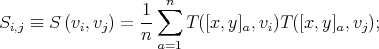 |
(6) |
n is the number of
positions in the map. The matrix Si,j contains
information about the distribution of all emitting velocities, but averages
out spatial information. The analysis uses Si,j to
find an orthogonal normalized basis set of eigenvectors that describes the
velocity distribution. A typical cloud may need only a few
eigenvectors; a field of CO emission in NGC 7538 needed only seven
components before the level of variation was comparable to the noise
(Brunt & Heyer
2002).
Brunt & Heyer
(2002)
used this
technique to determine the average scaling between correlations in
velocity and position, obtaining a power law with a slope of
~ 0.6 for several CO sources. Their fractal Brownian motion
models of clouds then suggested the intrinsic slope was ~ 0.5.
More recent studies comparing observations to simulations suggest
the slope is 0.5 to 0.8, which implies a steep energy spectrum,
E(k)
k-2
to k-2.6, although there are some ambiguities in the
method
(Brunt et al. 2003).
Velocity channel analysis was developed by Lazarian & Pogosyan (2000) to make use of the fact that the power spectrum of emission from a turbulent gas has a shallower slope in narrow velocity channels than in wide channels. This is a general property of correlated velocity fields. The shallow slope is the result of an excess of small features from unrelated physical structures that blend by velocity crowding on the line of sight. This blending effect has been studied and substantially confirmed in a number of observations (Dickey et al. 2001, Stanimirovic & Lazarian 2001) and simulations (Ballesteros-Paredes, Vázquez-Semadeni & Scalo 1999; Pichardo et al. 2000; Lazarian et al. 2001; Esquivel et al. 2003). Miville-Deschênes, Levrier & Falgarone (2003) noted that the method would not give the correct intrinsic power spectrum if the velocity channels were not narrow enough. If there are no velocity fluctuations, then the power spectrum of projected emission from a slab that is thinner than the inverse wave number is shallower than the 3D density spectrum by one (Goldman 2000, Lazarian et al. 2001).
Emission-line profiles also contain information about interstellar turbulence. Molecular cloud observations suggest that profile width varies with size of the region to a power between 0.3 and 0.6 (e.g., Falgarone, Puget & Perault 1992; Jijina, Myers & Adams 1999). Similar scaling was found for H I clouds by Heithausen (1996). However other surveys using a variety of tracers and scales yield little correlation (e.g., Plume et al. 1997, Kawamura et al. 1998, Peng et al. 1998, Brand et al. 2001, Simon et al. 2001, Tachihara et al. 2002), or yield correlations dominated by scatter (Heyer et al. 2001). An example of extreme departure from this scaling is the high resolution CO observation of clumps on the outskirts of Heiles Cloud 2 in Taurus, with sizes of ~ 0.1 pc and unusually large linewidths of ~ 2 km s-1 (Sakamoto & Sunada 2003). Overall, no definitive characterization of the linewidth-size relation has emerged.
Most clouds with massive star formation have non-Gaussian and irregular line profiles, as do some quiescent clouds (MBM12 - Park et al. 1996, Ursa Majoris - Falgarone et al. 1994, Figure 2b,c), while most quiescent clouds and even clouds with moderate low-mass star formation appear to have fairly smooth profiles (e.g., Padoan et al. 1999, Figure 4 for L1448). Broad faint wings are common (Falgarone & Phillips 1990). The ratios of line-wing intensities for different isotopes of the same molecule typically vary more than the line-core ratios across the face of a cloud. However, the ratio of intensities for transitions from different levels in the same isotope is approximately constant for both the cores and the wings (Falgarone et al. 1998; Ingalls et al. 2000; Falgarone, Pety & Phillips 2001).
Models have difficulty reproducing all these features. If the turbulence correlation length is small compared with the photon mean free path (microturbulence), then the profiles appear flat-topped or self-absorbed because of non-LTE effects (e.g., Liszt et al. 1974; Piehler & Kegel 1995 and references therein). If the correlation length is large (macroturbulence), then the profiles can be Gaussian, but they are also jagged if the number of correlation lengths is small. Synthetic velocity fields with steep power spectra give non-Gaussian shapes (Dubinski, Narayan & Phillips 1995).
Falgarone et al. (1994) analyzed profiles from a decaying 5123 hydrodynamic simulation of transonic turbulence and found line skewness and wings in good agreement with the Ursa Majoris cloud. Padoan et al. (1998, 1999) got realistic line profiles from Mach 5-8 3D MHD simulations having super-Alfvénic motions with no gravity, stellar radiation, or outflows. Both groups presented simulated profiles that were too jagged when the Mach numbers were high. For example, L1448 in Padoan et al. (1999; Figures 3 and 4) has smoother 13CO profiles than the simulations even though this is a region with star-formation. Large-scale forcing in these simulations also favors jagged profiles by producing a small number of strong shocks.
Ossenkopf (2002) found jagged structure in CO line profiles modelled with 1283 - 2563 hydrodynamic and MHD turbulence simulations. He suggested that subgrid velocity structure is needed to smooth them, but noted that the subgrid dispersion has to be nearly as large as the total dispersion. The sonic Mach numbers were very large in these simulations (10-15), and the forcing was again applied on the largest scales. Ossenkopf noted that the jaggedness of the profiles could be reduced if the forcing was applied at smaller scales (producing more shock compressions along each line of sight), but found that these models did not match the observed delta-variance scaling. Ossenkopf also found that subthermal excitation gave line profiles broad wings without requiring intermittency (Falgarone & Phillips 1990) or vorticity (Ballesteros-Paredes, Hartmann & Vázquez-Semandini 1999), although the observed line wings seem thermally excited (Falgarone, Pety & Phillips 2001).
The importance of unresolved structure in line profiles is unknown. Falgarone et al. (1998) suggested that profile smoothness in several local clouds implies emission cells smaller than 10-3 pc, and that velocity gradients as large as 16 km s-1 pc-1 appear in channel maps. Such gradients were also inferred by Miesch et al. (1999) based on the large Taylor-scale Reynolds number for interstellar clouds (this number measures the ratio of the rms size of the velocity gradients to the viscous scale, LK, see Section 4.2). Tauber et al. (1991) suggested that CO profiles in parts of Orion were so smooth that the emission in each beam had to originate in an extremely large number, 106, of very small clumps, AU-size, if each clump has a thermal linewidth. They required 104 clumps if the internal dispersions are larger, ~ 1 km s-1. Fragments of ~ 10-2 pc size were inferred directly from CCS observations of ragged line profiles in Taurus (Langer et al. 1995).
Recently, Pety & Falgarone (2003) found small (< 0.02 pc) regions with very large velocity gradients in centroid difference maps of molecular cloud cores. These gradient structures were not obviously correlated with column density or density, in which case they would not be shocks. They could be shear flows, as in the dissipative regions of subsonic turbulence. Highly supersonic simulations have apparently not produced such sheared regions yet. Perhaps supersonic turbulence has this shear in the form of tiny oblique shocks that simulations cannot yet reproduce with their high numerical viscosity at the resolution limit. Alternatively, ISM turbulence could be mostly decaying, in which case it could be dominated by low Mach number shocks (Smith, Mac Low & Heitsch 2000; Smith, Mac Low & Zuev 2000).