1. SFR DETERMINATIONS FROM SED MODELLING

During this meeting we have discussed a lot about different methods of deriving star formation rates in galaxies and what the advantages and disadvantages of using different calibrations are (see the comprehensive review talk by Veronique Buat at this meeting; see also review by Calzetti 2012). During the session on SFR determinations from SED modelling, but also throughout the meeting, two SED modelling approaches have been presented and discussed: the energy balance method and the radiative transfer modelling.

The energy balance method relies on the conservation of energy between the stellar light aborbed by dust and that emitted (by the same dust) in the mid-IR/far-IR/submm. This is by far a superior method to only fitting SED templates in a limited spectral range (see talk by Denis Burgarella). Nonetheless, the energy-balance method is not a self-consistent analysis, since the SED of dust emission is not calculated according to the radiation fields originating from the stellar populations in the galaxy under study, but rather according to some templates. The templates can be either empirical (Xu et al. 1998, Devriendt et al. 1999, Sajina et al. 2006, Marshall et al. 2007) or theoretical (Dale & Helou 2002, Draine & Li 2007, Natale et al. 2010). At this meeting we saw applications of two energy balance methods, MAGPHYS (da Cuhna et al. 2008) and CIGALE (Burgarella et al. 2005, Noll et al. 2009). The energy balance method is a useful tool when dealing with large statistical samples of galaxies for which little information is available regarding morphology/type, orientation and overall size. This advantage comes nevertheless with the disadvantage that the energy balance methods cannot take into account the effect on the dust attenuation and therefore also on the dust emission of the different geometries of stars and dust present in galaxies of different morphological types, neither can it take into account the anisotropies in the predicted stellar light due to disk inclination (when a disk geometry is present). These methods can therefore only be used in a statistical sense, when dealing with overall trends in galaxy populations.

The radiative transfer method is the only one that can self-consistently calculate the dust emission SEDs based on an explicit calculation of the radiation fields heating the dust, consequently derived from the attenuated stellar populations in the galaxy under study. At this meeting we saw applications of the RT model of Popescu et al. (2011). This method can take advantage of the constraints provided by available optical information like morphology, disk-to-bulge ratio, disk inclination (when a disk morphology is present) and size. As opposed to the energy balance method, this advantage comes with the disatvantage that such information is not always easily available. Nonetheless these radiation transfer methofs could perhaps be adapted to incorporate this information (when missing) in the form of free parameters of the model, though such attempts have not yet been made. Another drawback of these methods was that radiative transfer calculations are notorious for being computationally very time consuming, and as such, detailed calculations have been mainly used for a small number of galaxies (Popescu et al. 2000, Misiriotis et al. 2001, Popescu et al. 2004, Bianchi 2008, Baes et al. 2010, MacLachlan et al. 2011, Schechtman-Rook et al. 2012, de Looze et al. 2012a, b). This situation has been recently changed, with the creation of large libraries of radiative transfer model SEDs, as performed by Siebenmorgen & Krugel (2007) for starburst galaxies, Groves et al. (2008) for star-forming regions/starburt galaxies and Popescu et al. (2011) for spiral galaxies.

Reviews on determination of star-formation in galaxies have so far not included discussions on the use of radiative transfer methods, with the exception of the review of Kylafis & Misiriotis (2006) With the new developments resulting in the creation of libraries of RT models, we can now start to include radiative models as main topics of discussion. Indeed, at this meeting we emphasised that they are in fact the most realible way of deriving star formation rates in galaxies. In this way the SFRs are derived self-consistently using information from the whole range of the electromagnetic spectrum, from the UV to the FIR/submm, incorporating information with morphological constraints (primarily from optical imaging). Here we did not consider radio and Xray emission, though these emissions have been discussed in other sessions of this meeting (e.g. talk by Bret Lehmer). In particular the SED modelling has been discussed in conjunction with the most difficult cases, namely those of translucent galaxies: galaxies with both optically thin and thick components. In one way optically thin galaxies are more easily dealt with, since most of the information on SFR can be derived from the UV. Very optically thick cases are also easy from this point of view, since SFR can be derived from their FIR emission, providing one can isolate the AGN powered emission. But the most difficult cases are the translucent galaxies. These are essentially the spiral galaxies in the Local Universe, and probably a large fraction of the star forming dwarf galaxies - which dominate the population of galaxies in the Local Universe, and which also host most of the star formation activity taking place in the local Universe. We showed in this meeting how important it is to quantify this star formation activity. We also discussed how important it is to quantify the star formation activity in the high redshift Universe; it is just that for the moment we do not have enough detailed information to be able to do the same type of analysis that we can now do for the Local Universe. Here I will summarise the main points we addressed:

1. Why is it so difficult to calibrate SFR in spiral galaxies and why do we need to follow the fate of photons with radiative transfer calculations?

• Fundamentally, any fixed observed luminosity in dust emission can be powered either by a small fraction of a large quantity of optical light from older stellar populations, or by a large fraction of a small quantity of UV light from younger stellar populations. Only radiation transfer techniques can unravel this dichotemy.

• Because of the disky nature of these systems, the direct UV and optical light is highly anisotropic, and the attenuation of the stellar photons will depend on the viewing angle and wavelength. Fig. 1 illustrates the strong dependence of the observed luminosity of stellar disks on the viewing angle.

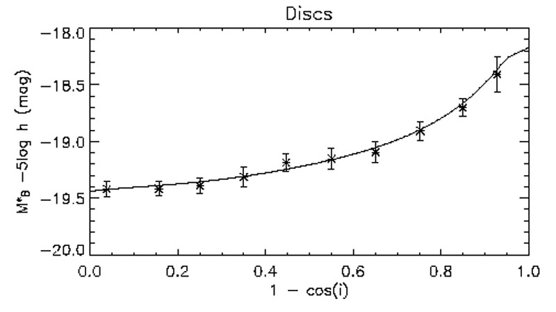  Figure 1. The attenuation-inclination relation from Driver et al. (2011). The symbols deliniate the empirical relation derived for disks from the Millenium Galaxy Survey while the solid line is the prediction from the model of Tuffs et al. (2004).

• Dust in galaxies has a very complex structure, containing both diffuse components on kiloparsec scales, as well as localised components, at the pc scales, associated with the star forming regions. The escape of radiation from these two components is very different, as it is the heating of dust in the diffuse medium and in the star-forming clouds.

• Disk galaxies have different morphological components, in particular disks and bulges. The attenuation characteristics of disks is very different from those of bulges (see Fig. 2) and these need to be properly taken into account when dealing with the integrated emission from galaxies.

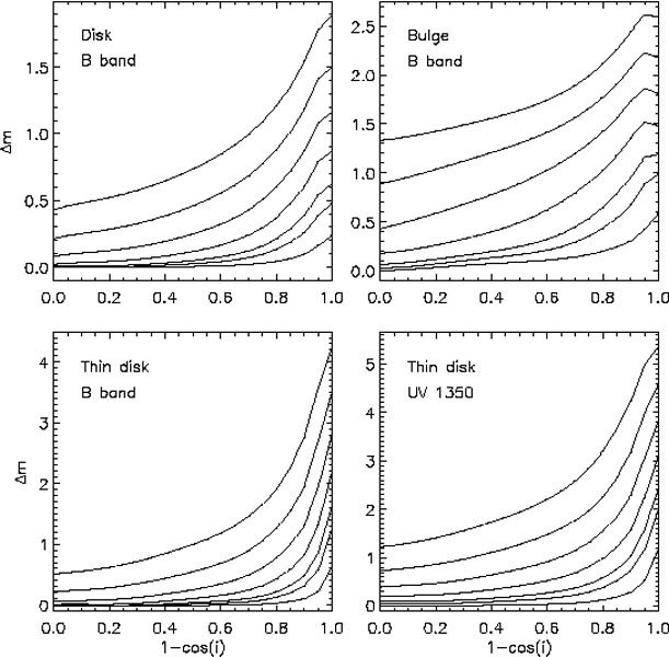  Figure 2. Predictions for the attenuation-inclination relation for different stellar components from Tuffs et al. (2004). From bottom to top the curves correspond to central face-on B band optical depth Bf of 0.1, 0.3, 0.5, 1.0, 2.0, 4.0, 8.0

• Different stellar populations have different spatial distributions with respect to the dust distribution, and again their attenuation characteristics will differ, as will their contribution to heating the dust. Fig. 2 illustrates the different behaviour of the variation of attenuation of light coming from different stellar populations with inclination and dust opacity. Fig. 3 also shows how the dust and PAH emission SEDs are changed for various contributions coming from the old and young stellar populations in the disk, as well as from the old stellar populations in the bulge.

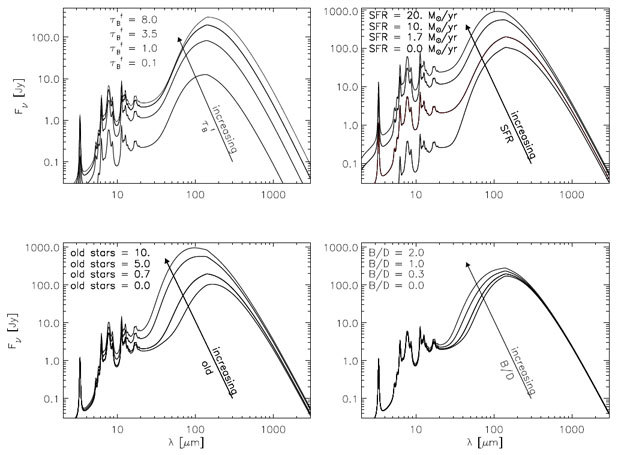  Figure 3. Predictions for dust and PAH emission SEDs based on the model of Popescu et al. (2011). In going clock-wise from the top-left, the different panels show the effect of changing the dust opacity, the luminosity of the young stellar populations (SFR), the luminosity of the old stellar populations (old) and the bulge-to-disk (B/D) ratio. In each panel only one parameter at a time is changed, while keeping the remaining ones fixed.

2. Why do SFR calibrators work?

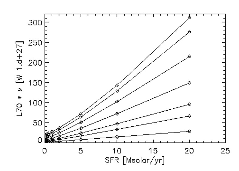
SED modelling tools based on self-consistent radiative transfer calculations can be used to predict the scatter in the SFR calibration relations, as a function of the main intrinsic parameters that can affect these relations. Several of these relations have been presented. In Fig. 4 we only show predictions for the SFR calibration based on monochromatic FIR luminosities when the dust opacity changes. The predictions are based on the model of Popescu et al. (2011). The figure shows a very large scatter in the correlations. A similar large scatter is predicted for correlations corresponding to various contributions coming from the old stellar populations, or for the clumpiness of the ISM. For the UV calibrators large scatters are also predicted when some of the relevant parameters (viewing angle, dust opacity, bulge-to-disk ratio and clumpiness of the ISM) vary. Overall it is apparent from these plots that the predicted scatter in the SFR correlations due to a broad range in parameter values is larger than observed in reality. The question then arises of why are the SFR calibrators working, despite, for example, the very crude dust corrections that have been so far used in the community? A possible answer is the existence of some scaling parameters, which do not allow a continuous variation in parameter space, in particular for dust opacity or stellar luminosity. Recent work from Grootes et al. (2013) proved the existence of a well-defined correlation between dust opacity and stellar mass density. The correlation was derived on data coming from Galaxy and Mass Assembly (GAMA) survey (Driver et al. 2011) and the Herschel ATLAS survey (Eales et al. 2011), in combination with the model of Popescu et al. (2011). These finding give support to the interpretation of the existence of fundamental physical relations that reduce the scatter in the SFR correlations.

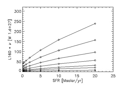Figure 4. Predictions for the relation betwween the 70 µm (left) and 160 µm luminosity versus SFR based on the model of Popescu et al. (2011). From bottom to top the curves correspond to central face-on B band optical depth values of 0.1, 0.3, 0.5, 1.0, 2.0, 4.0 and 8.0.

3. A word of caution

We have identified some points where things should be treated more carefully in the future:

• The energy balance method should not be used on scales smaller than the scalelength of the disk, as the energy is not conserved below these scales. The role of long range photons in the diffuse ISM should not be underestimated, in particular by considering an average free path of photons in the disk. This is because the free path of photons firstly depends on radial position in the galaxy (disk), where dust opacity is known to decrease monotonically with radius (e.g. Boissier et al. 2004, Popescu et al. 2005). Secondly, there is also a vertical distribution of dust, and the free path of photons in vertical direction will be different from that in radial direction. One also needs to add the contrast between arm and interarm regions. Finally, the escape of photons from star-forming clouds is strongly anisotropic and fragmented, because of the fragmentation of the clouds themself. Thus, in some directions the stellar light is completely absorbed by dust, while there are lines of sight from which the radiation freely escapes in the surrounding diffuse medium. The multiple facets of the transfer of radiation in galaxies, including the effect of scattered light, means that energy balance method should not be applied on a pixel by pixel basis, as sometimes employed in the literature.

• Mid-IR emission should not only be identified with "small grain" emission, where by small grain we mean stochastically-heated grains. In fact in the range 24-60 µm most of the dust emission is powered by big grains heated at equilibrium temperatures by the strong radiation fields in the star-forming complexes.

• The ratio between mid-IR (PAH range) emission to FIR emission cannot be interpreted only in terms of relative abundances of PAH to big grains. One should also take into account the change in the colour and intensity of the radiation fields heating the dust, which also result in strong variations of mid-IR to FIR emission.

• Do we really need to accurately know the absolute star-formation rates in galaxies? Perhaps we can live with some approximations, which would be good enough to allow us to derive trends in galaxy populations over cosmic time. A definitive no has been given to this suggestion. An inability to measure absolute SFR would severely limit our ability to constrain physical models of galaxies and the evolving universe. For example, only if we have absolute measurements of SFR will we be able to relate measurements of SFR to measurements of gas content of galaxies in terms of physical models predicting the amount of gas in the ISM and the efficiency of conversion of the ISM into stars. Pavel Kroupa also gave convincing statistical argumentation on the need to measure accurate SFRs in the discussion session.

4. What else have we learned?

• Applications of self-consistently calculated model SEDs strongly rely on scaling them according to measurements of the surface area of the stellar disk of the modelled galaxy, which, in turn, depends on an accurate decomposition of the main morphological components of galaxies as observed in the UV/optical. Bogdan Pastrav showed that the derived scale-sizes of stellar disks of galaxies are strongly affected by dust (see Fig. 5), and that a proper determination of the intrinsic distributions of stellar emissivity, and thus of star-formation rates, needs to self-consistently take into account these effects.

  Figure 5. Dust effects on the derived scalelength of disks fitted with exponential functions (left) and on the derived effective radius of disks fitted with variable index Sérsic functions, from Pastrav et al. (2013)>. Both plots are for the B band. From bottom to top curves are for a central face-on dust opacity in the B band of 0.1, 0.3, 0.5, 1.0, 2.0, 4.0, 8.0.

• Several panchromatic surveys, with detailed information on bulge-to-disk ratio, inclination and disk size are underway, making these databases ideal for determinations of SFR using radiative transfer models. Andreas Zezas presented "The Star-Formation Reference Survey" (Ashby et al. 2011), a unique statistical sample of 369 galaxies selected to cover all types of star-forming galaxies in the nearby universe. The survey overlaps with the SDSS and NVSS areas and has GALEX, SDSS, 2MASS, Spitzer and NVSS multiband photometry and planned bulge-disk decompositions of optical images, which will make it ideal for self-consistent and systematic determinations of SFRs. It will also asses the influence of AGN fraction and environment on SFR.

• Denis Burgarella presented applications of the CIGALE SED fitting method on the Lyman break galaxies at 2.5 < z < 4 detected in the Far-infrared with Herschel and implication for star formation determinations at high redshift.

• Andrew Hopkins showed results on SFRs derived from applications of the energy balance method on the GAMA survey. Applications of radiative transfer techniques to the de-reddening of GAMA galaxies by Grootes et al. (2013) were presented in the review of C. Popescu.