Copyright © 2014 by Annual Reviews. All rights reserved
| Annu. Rev. Astron. Astrophys. 2014. 54:
Copyright © 2014 by Annual Reviews. All rights reserved |


The fundamental observable for a radio interferometer is the arrival time
difference of wavefronts between antennas, owing to the finite
propagation speed of electro-magnetic waves (the speed of light c).
For an ideal interferometer, the arrival time difference is determined
by the locations of the antennas with respect to the line-of-sight to
the source and is referred to as the "geometric delay." The basic
equation of a radio interferometer,
which relates the geometric delay, τg, to the source unit
vector,  , and the
baseline vector,
, and the
baseline vector,  ,
is given by
,
is given by
 |
(1) |
In Figure 7, we sketch the geometry of these
vectors. Note that while the source vector
has two parameters
(e.g., right ascension and declination), the geometric delay is a scalar
and so multiple measurements of
geometric delays are required to solve for a source position.
Such measurements can be made, even with a single baseline, by utilizing
the Earth's rotation, which changes the orientation of the baseline
vector with respect to the celestial frame.
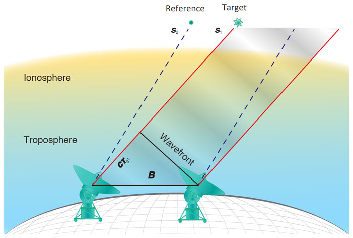 |
Figure 7. Schematic view of a delay measurement in phase-referencing astrometry. Here, for simplicity, an array with two stations is shown. The baseline vector and source directions are indicated by lines. In relative astrometry, the target and adjacent reference sources are observed (nearly) at the same time so delay errors can be effectively canceled in the relative measurement. For relative radio astrometry, the dominant error sources are generally uncompensated propagation delays in troposphere and/or ionosphere. |
We now consider the effects of observational errors on astrometric accuracy. Given the uncertainty in a delay measurement, which we denote Δτ, from Equation 1 one can roughly estimate the astrometric error, Δ s:
 |
(2) |
As seen in Equation 2, for a given Δτ, astrometric accuracy improves with longer baselines. This is the fundamental reason why VLBI, which utilizes continental and/or inter-continental baselines, can achieve the highest accuracy astrometry. For example, for an 8,000 km baseline and a typical delay error of ~ 2 cm (converted to path length by cΔτ), one expects an astrometric error of ~ 0.5 mas. This is a typical error for absolute astrometry, such as measuring QSO positions in the ICRF using broad-band delay measurements.
For Galaxy-scale parallaxes, however, this accuracy is insufficient as parallaxes can be ~ 0.1 mas, corresponding to distances of ~ 10 kpc. At such distances, one needs astrometric accuracy of ± 10 μas to achieve ± 10% uncertainty. In order to obtain μas-level accuracy, one must substantially cancel systematic delay errors through relative astrometry, i.e., a position measurement with respect to a nearby reference source. Historically, the concept of relative astrometry has been attributed to Galileo, who proposed measuring the parallax of a nearby star with respect to a more distant star located close by on the sky.
The delay measured with an interferometer can be considered as the sum of the geometric delay (which we would like to know) and additional terms (which need to removed from the data):
 |
(3) |
Here τtropo and τiono are the delays in the propagation of the signal through the troposphere and ionosphere, respectively, τant is caused by an error in the location of an antenna, τinst is an instrumental delay in the telescope or electronics, τstruc is the delay due to unmodeled source structure, and τtherm is the uncertainty in measuring delay caused by thermal noise. Note that generally throughout this review the terms "delay" and "phase" (or phase-delay) can be used interchangeably: for instance, the interferometric phase caused by the geometric delay in Equation 1 can be written as,
 |
(4) |
where ν is the observing frequency.
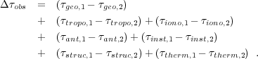
For relative astrometry, one observes two sources, the target and reference, at nearly the same time and nearly the same position on the sky, and differences the observed delays (phases) between the pair of sources. This type of observation is often referred to as "phase-referencing," as the observed phase of the reference source is used to correct the phase of the target. Applying Equation 3 for the difference between two sources, we obtain the delay difference observable:
 |
(5) |
Here subscripts 1 and 2 denote the quantities for the target and reference source, respectively. The first term is the difference in geometric delay between the source and reference, which corresponds to the relative position of the target source with respect to the reference source. The additional terms in the Equation 5 may be reduced if they are similar for the two lines of sight. As will be discussed in detail later, four terms (τtrop, τiono, τstar, and τinst) are antenna-based quantities (delays originated at each antenna) and generally are similar for the target and reference lines of sight, for small source separations.
Antenna-based terms can be effectively reduced by phase-referencing.
For example, the delay error generated by an antenna position offset,
Δ, is given by
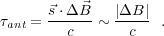 |
(6) |
Note the approximation used to obtain the right hand side of Equation 6
is that the trigonometric terms in the vector dot product are generally
 1.
Differencing the antenna delays for two adjacent sources, yields
1.
Differencing the antenna delays for two adjacent sources, yields
 |
(7) |
where θsep is the separation angle between the sources. Comparison of Equations 6 and 7 shows that the delay error caused by an antenna position error is reduced by a factor of θsep in the differenced delay. This reduction can significantly improve relative over absolute astrometric accuracy. For a separation of θsep = 1°, the error reduction factor (θsep) is about 0.02 (radians).
As we will discuss later in more detail, the dominant error source in
radio astrometry is uncompensated propagation delays, generally tropospheric
for observing frequencies
 10 GHz and
ionosphere for lower frequencies. These terms are "antenna-based," just
as the antenna location errors described above.
A rough estimate of astrometric accuracy achievable in the presence of
propagation delay errors is given by
10 GHz and
ionosphere for lower frequencies. These terms are "antenna-based," just
as the antenna location errors described above.
A rough estimate of astrometric accuracy achievable in the presence of
propagation delay errors is given by
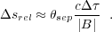 |
(8) |
The reduction in position uncertainty in going from Equation 2 to Equation 8 is, of course, the addition of the canceling term, θsep. Using the same example values previously used for absolute astrometry, (|B| = 8000 km and a delay error of cΔt ~ 2 cm), relative astrometric accuracy for a 1° source separation is ~ 10 μas.
Uncompensated delay differences between antennas in an interferometric array usually limit radio astrometric accuracy. In this subsection, we discuss sources of delay errors individually.
4.2.1 TROPOSPHERE The propagation speed of electro-magnetic waves in the troposphere is slower than in vacuum, causing an extra delay (τtropo) to be added to the geometric delay. The tropospheric delay is almost entirely non-dispersive (frequency independent) at radio frequencies. It is convenient to separate the tropospheric delay into two components based on the timescales of fluctuation: a slowly (~ hours) and rapidly (~ minutes) varying term.
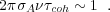
The rapidly varying term is associated with the passage of small "clouds" of water vapor flowing at wind speeds of ~ 10 m s-1 at a characteristic height of ~ 1 km over each antenna. This can be the main cause of coherence loss in interferometric observations. The characteristic time scales for interferometer phase fluctuations induced by tropospheric water vapor can be described by the Allan standard deviation (σA) and is typically ~ 0.5 to 1 × 10-13 over timescales of 1 to 100 sec (Thompson, Moran & Swenson 2001, Honma et al. 2003). An interferometer coherence time, τcoh, can be defined as the time interval over which phase fluctuation differences between two antennas accumulate one radian. At an observing frequency ν, this implies
 |
(9) |
For σA = 0.7 × 10⁻¹³ and ν = 22 GHz, this implies a coherence time of ~ 100 sec. One must measure and remove the phase variations on a time-scale shorter than the coherence time. Rapid switching between the target and calibrator sources can usually accomplish this, provided the antennas can slew and settle on sources rapidly (see Section 4.3).
The rapid variations from tropospheric delays can be completely removed if one can simultaneously observe the target and calibrate sources . This is done with the VERA antennas, which have dual-beam observing systems. Alternatively, this can also be accomplished if one is fortunate in finding a source pair with a very small angular separation, so that both fit within the primary beam of the antennas ("in-beam" calibration). Note that with either method, this still leaves a spatial variation component, but that term is generally smaller than the temporal term for source separations of a few degrees.
The slowly varying delay term is generally associated with the "dry" part of the troposphere, although the slow term can also contain a small, relatively stable contribution from water vapor. At sea-level, a typical path delay for the dry component is 230 cm at the zenith and water vapor can contribute up to a several tens of cm for very humid locations. The total dry delay can be estimated from antenna latitude and elevation, and if necessary using local temperature and pressure values. Since the total dry delay is considerable, it is important to remove its effects during correlation, or early in post-correlation processing, by carefully accounting for the exact slant path through the atmosphere (air mass), which will be different for the target and calibrator. The slowly varying wet component cannot reliably be estimated from surface weather parameters and needs to be directly measured and removed to achieve μas astrometry (see Section 5.1.1 and Section 5.1.2 for details).
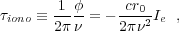
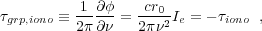
4.2.2 IONOSPHERIC DELAY The ionosphere is a partially ionized layer located between ~ 50 and ~ 500 km altitude. An electromagnetic wave propagating through this plasma experiences phase and group delays that are frequency dependent (i.e., dispersive delays). The phase and group delay are given by
 |
(10) |
and
 |
(11) |
where r0 is the classical electron radius and Ie = ∫ne dl is the electron column density along the line of sight or total electron content (TEC). Due to the dispersive nature of plasma, delays are larger at lower frequency because of the ν-2 dependence. (Note that the ionospheric phase delay has the opposite sign of the group delay; therefore correction of interferometer phase for ionospheric delays is different than for tropospheric delays.)
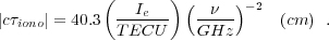
The ionization of the ionosphere is predominantly from solar radiation, and thus there is a strong diurnal variation, as well as from the 11 year solar cycle. Due to the diurnal variation, the ionospheric delay needs to be modeled (or measured) and calibrated on hour scales. Modeling of the ionospheric delays is done by a combination of a vertical TEC (VTEC) and a mapping (air mass like) function. Typical values for VTEC range from a few to 100 TECU, where 1 TECU corresponds to an electron column density of 1016 m-2. Once the TEC toward a source is known, the ionospheric delay (in path length units) can be calculated by the following relation,
 |
(12) |
At a frequency of 22 GHz, a 50 TECU column density causes a delay equivalent to an extra path length of ~ 4 cm, but it reaches ~ 400 cm at a frequency of 2 GHz.
Because of the dispersive nature of the ionospheric delay, dual-frequency observations are effective for calibration. Most geodetic measurements involve simultaneous observations at 2.3 and 8.4 GHz in order to calculate and then remove ionospheric delays. Another way to measure ionospheric TEC values is to use GPS data, which provide dual-frequency signals at 1.23 and 1.58 GHz. Several services accumulate GPS data from stations around the Earth and provide global TEC models approximately every two hours. Generally, radio interferometric data are calibrated for ionospheric delays using these models.
4.2.3 INSTRUMENTAL DELAY
Radio propagation in antenna structures, feeds, and electronics causes
additional delays, which we lump together as "instrumental delays"
(τinst).
In addition, there are electronic phase offsets associated with the
generation of the local oscillators used to mix the observed frequencies
to "intermediate" frequencies (~ 1 GHz) prior to correlation.
The data recorded at each antenna are time-tagged using a clock tied to
the fundamental frequency standard at each station
(usually a hydrogen maser atomic oscillator),
and owing to slight frequency offsets (that do not affect local oscillator
stability) these clocks generally gain or lose time at a rate of one
part in ~ 10-14 (only ~ 1 nsec per day!).
However, a delay error of 1 nsec causes a phase
slope of π radians across a 500 MHz observational bandwidth, and it is
critical to correct for this. Calibration observations using "geodetic
blocks" (see Section 5.1.1) can remove
clock errors to an accuracy of
0.1 nsec.
Other instrumental delay and phase offsets are generally relatively
slowly varying,
for well designed systems and temperature controlled electronics, and can be
calibrated and removed by observations of strong sources a few times a day.
Any residual instrumental delay and phase offsets will be mostly canceled when switching between two sources, provided the electronics are not changed. Note that if one of the sources is a spectral line and the other a continuum emitter, one should try to place the line near the center of the continuum band to ensure better calibration. On the other hand, if the two sources are observed with different receivers, which is the case for dual-beam receiving at VERA, there is a need for additional calibration of the instrumental delay and phase, such as by using an artificial noise source (see Section 4.3).
4.2.4 ANTENNA POSITION
The antenna position is usually defined as the intersection
of azimuth and elevation axes and can be measured to an accuracy
of 3 mm with
regular geodetic observations.
The Earth's rotation rate varies (measured as a time correction, UT1-UTC)
as does the location of an antenna on the Earth's crust with respect to
its spin axis (polar motion). Together these are called Earth
Orientation Parameters (EOP). EOP values are determined on a daily basis
by the International Earth Rotation and Reference Systems Service (IERS)
by utilizing global GPS data and geodetic VLBI observations.
A typical error in EOP values is ≈ 0.1 mas, provided
the final (not preliminary or extrapolated) values are used.
With high accuracy antenna locations and EOP corrections, the total
uncertainty in the position of an antenna contributes less to the
astrometric error budget than uncertainty in atmospheric propagation delays.
4.2.5 SOURCE STRUCTURE If the observed sources are not point like, interferometric delay/phase can be affected by source structure. Since structure phase shifts are independent for the target and reference sources, their effects do not cancel when differencing the phases in relative astrometry. Source structure phases are baseline-based quantities. Because there are ~ N2 baselines for N antennas in an array, structure phase can be separated from station-based quantities and estimated using self-calibration (closure techniques and hybrid-mapping). Once a source image is obtained, phase shifts caused by source structure can be calculated and subtracted from observed interferometric data. Note that since self-calibration loses absolute position information, if one self-calibrates the reference source data, one must apply the same calibrations to both the reference and target source to preserve relative astrometric accuracy. Generally it is not a good idea to self-calibrate the target source data, but instead measure the structure in the phase-referenced images.
4.2.6. THERMAL NOISE Thermal (usually dominated by receiver) noise is random and cannot be calibrated and removed. However, a random process does not cause systematic offsets, and by integrating over many samples its effects can be reduced. Thermal noise in an interferometric image leads to position measurement uncertainty given by Equation 1 of Reid et al. (1988):
 |
(13) |
For a baseline length B = 8000 km and observing wavelength λ = 1.3 cm, the synthesized beam (FWHM) size is θbeam ≈ 0.3 mas. Thus, for a source with an image signal-to-noise ratio SNR ~ 30, the expected position error due to thermal noise is only ≈ 5 μas. Therefore, thermal noise often is not a major source of radio astrometric error.
Several methods of phase-referencing are commonly used:
source switching, dual-beam, and in-beam observations.
Source switching or "nodding" is the most-commonly used observing method,
because it does not require a special radio telescope and can be used
for all source pairs. The only requirement is that slewing/settling
times are short enough to track tropospheric phase fluctuations.
As discussed in Section 4.2.1, coherence times at
an observing
frequency of 22 GHz are ~ 100 sec. Therefore switching cycles should be
shorter than this time, e.g., a cycle of 60 sec obtained by integrating for
20 sec on the reference, 10 sec for slewing to the target, integrating
for 20 sec on the target, then 10 sec for slewing back to the reference.
Because of the non-dispersive nature of tropospheric delays, the
interferometer coherence time scales linearly with wavelength,
i.e., τcoh ∝ λ.
Hence at a short wavelengths, the coherence time can be problematic.
For an observing wavelength of λ = 1.3 mm (ν = 230 GHz),
the coherence time is likely to be ~ 10 sec. This makes it practically
impossible to conduct switched VLBI observations at
1 mm wavelength.
In dual-beam observations, two sources are observed simultaneously using independent feeds and receivers. This can be done using multi-feed systems on a single antenna, as with VERA, or with multiple antennas at each site (Rioja et al. 2009, Broderick, Loeb & Reid 2011). There is no gap between the observations of the target and reference sources, and hence there is no coherence loss owing to temporal phase fluctuations. The antennas of the VERA array achieve this with two receivers installed at the Cassegrain focus. These receivers are independently steerable with a Steward-mount platform, and one can observe a source pair with separation angles between 0.3° to 2.2°. In dual-beam radio astrometry, special care needs to be taken to calibrate the instrumental delay, because it is not common to the target and reference source and thus will not cancel when phase-referencing.
In-beam observations can be regarded as a special case of phase-referencing, where the target and reference sources are so closely located that the two sources can be observed simultaneously with a single feed (within the primary beam of each antenna). In such a case, calibration error can be very effectively reduced, because the observations are done at the same time for the target and reference, and, because the separation angle is small, most systematic errors are largely canceled. However, finding a sufficiently strong reference source may be difficult; as such in-beam observations are more common at lower observing frequencies, as the primary beam becomes larger and the reference sources stronger.