4. THE REDSHIFTED 21 CM AS A PROBE OF THE EoR

In recent years it has become clear that the 21 cm line can be used to probe the neutral IGM prior to and during the reionization process. This hyperfine transition line of atomic hydrogen (in the ground state) arises due to the interaction between the electron and proton spins [83, 180, 120]. The excited triplet state is a state in which the spins are parallel whereas the spins at the lower (singlet) state are antiparallel. The 21 cm line is a forbidden line for which the probability for a spontaneous 1→ 0 transition is given by the Einstein A coefficient that has the value of A₁₀ = 2.85 × 10^-15 sec^-1. Such an extremely small value for Einstein-A corresponds to a lifetime of the triplet state of 1.1 × 10⁷ years for spontaneous emission. Despite its low decay rate, the 21 cm transition line is one of the most important astrophysical probes, simply due to the vast amounts of hydrogen in the Universe [58, 209, 139] as well as the efficiency of collisions and Lyman- radiation in pumping the line and establishing the population of the triplet state [215, 61]. In this chapter I will describe the basic physics behind this transition, especially what decides its intensity.

4.1. The 21 cm Spin and Brightness Temperatures

The intensity of the 21 cm radiation is controlled by one parameter, the so called spin temperature, T_spin. This temperature is defined through the equation,

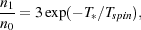(9)

where n₁ and n₀ are the number densities of electrons in the triplet and singlet states of the hyperfine level respectively, and T_∗ = 0.0681 K is the temperature corresponding to the 21 cm wavelength. The spin temperature is therefore, merely a shorthand for the ratio between the occupation number of the two hyperfine levels. This ratio establishes the intensity of the radiation emerging from a cloud of neutral hydrogen. Of course, in the measurement of such radiation one has to take into account the level of background being transmitted through a given cloud as well as the amount of absorption and emission within the cloud. Namely, one has to use the equation of radiative transfer.

In the following derivation I follow the description in Rybicki and Lightman ([173]). The radiative transfer equation is normally written in terms of the brightness (or specific intensity) of the radiation I. This quantity is defined as the intensity per differential frequency element in the form, I = dI / d, where is the frequency. The intensity has the dimensions of ergs s^-1 cm^-2 sr^-1 Hz^-1, namely, it quantifies the energy carried by radiation traveling along a given direction, per unit area, frequency, solid angle, and time. The radiative transfer equation for thermally emitting material at temperature T can be written in terms of the optical depth for absorption as,

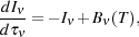(10)

where is the optical depth for absorption through the cloud at a given frequency and B is the Planck function.

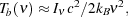
In radio astronomy the intensity I is often expressed by its equivalent brightness temperature, T_b(). This is convenient because at the Rayleigh-Jeans low energy limit, the relation between the brightness temperature and specific intensity is given by,

(11)

where c is the speed of light and k_B is the Boltzmann's constant. Expressing the radiative transfer equation 10 in terms of the brightness temperature gives it a particularly simple form,

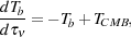(12)

where I substituted the CMB temperature for the background temperature. Solving equation 12 yields the temperature of the emergent radiation at frequency ,

(13)

where T_spin = T_b(0) is the brightness temperature in the absorbing cloud (see Figure 14). Notice that for the background radiation the factor exp(-) gives the transmission probability of the background radiation whereas the 1 - exp(-) factor gives the emission probability of 21 cm photons from within the cloud. Therefore, in order to determine the brightness temperature, one needs to know the optical depth for absorption, , and the spin temperature, T_spin, in the optically thin regime relevant to our case. Notice that in the case in which T_spin = T_CMB the brightness temperature gives exactly the CMB temperature. This is simply because in such a case there is a prefect balance between the absorption and emission at every frequency. Therefore, the measurement in such a case does not reveal anything interesting about the intervening cloud, the subject we are interested in here.

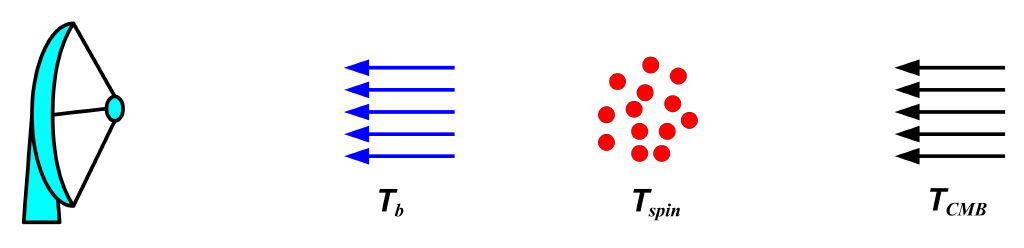Figure 14. A cartoon that shows that set up of the various components relevant to radiative transfer problem at hand starting from the background (CMB) radiation, going through a certain cloud with temperature Tspin and emerging with a temperature Tb that is measured by our telescopes.

I will first start with calculating the 21 cm optical depth. The hyperfine transition of atomic hydrogen is an ideal transition to be described by Einstein coefficients and their relations. The 21 cm radiation incident on the atom can cause 0 → 1 transitions (absorptions) and 1 → 0 transitions (induced emissions) corresponding to Einstein coefficient B₀₁ and B₁₀ respectively. The probabilities are given by,

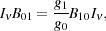(14)

and

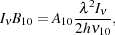(15)

respectively [173]. Here ₁₀ = 1420.4 MHz is the frequency of the 21 cm transition.

The 21 cm line absorption cross section is given by

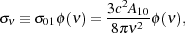(16)

where () is the line profile defined so that ∫d () = 1 and has units of time.

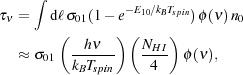
The optical depth of a cloud of hydrogen is then:

(17) (18)

where N_HI is the column density of H I and dℓ is a line element within the cloud. The factor of 4 connecting n₀ and H I accounts for the fraction of atoms in the hyperfine singlet state. The second factor in equation (17) with E₁₀ accounts for stimulated emission. The approximate form in equation (18) assumes uniformity throughout the cloud.

We now substitute for () and N_HI using cosmological quantities. In general, the line shape () includes natural, thermal, turbulent and velocity broadening, as well as bulk motion (which increases the effective Doppler spread). Velocity broadening is the most important effect in the IGM. Hubble expansion of the gas results in velocity broadening of a region of linear dimension ℓ will be v ~ ℓ H(z) so that () ~ c / (ℓ H(z) ). The column density along such a segment depends on the neutral fraction x_HI of hydrogen, so N_HI = ℓ x_HI n_H(z) [67]. A more exact solution of equation (17) yields an expression for the 21 cm optical depth of the diffuse IGM,

(19) (20)

where in the second relation, T_spin is in degrees Kelvin. Here the factor (1 + ) is the fractional overdensity of baryons and d v_|| / d r_|| is the gradient of the proper velocity along the line of sight, including both the Hubble expansion and the peculiar velocity [96]. In the second line, we have substituted the velocity H(z) / (1 + z) appropriate for the uniform Hubble expansion at high redshifts.

Next we need to calculate the spin temperature and substitute in Eq. 13. In his seminal papers, George Field [61, 62], used the quasi-static approximation to calculate the spin temperature, T_spin, as a weighted average of the CMB temperature, T_CMB, the gas kinetic temperature, T_kin, and the temperature related to the existence of ambient Lyman- photons, T [215, 62]. For almost all interesting cases, one can safely assume that T_kin = T [61, 67, 120, 135].

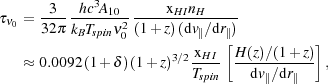
Three competing processes determine T_spin: (1) absorption of CMB photons (as well as stimulated emission); (2) collisions with other hydrogen atoms, free electrons, and protons; and (3) scattering of Lyman photons through excitation and deexcitation. Hence, the spin temperature could be recast as [61]:

(21)

where y_kin and y are the kinetic and Lyman- coupling terms, respectively. It is important to note that for the 21 cm radiation to be observed, it has to attain a different temperature than that of the CMB background [61, 63, 62, 83, 215]. The form I use here for Eq. 21 is the original form used in the George Field's 1958 paper [61], whereas some authors use a form that relates the inverse of the various temperatures. Both ways are of course equivalent but one needs to be careful with the definitions of the coupling coefficients in each case.

The kinetic coupling term y_kin is due to collisional excitations of the 21 cm transitions. The Lyman- coupling term y is due to the so called Lyman- pumping mechanism, also known as the Wouthyusen-Field effect, which is produced by photo-exciting the hydrogen atoms to their Lyman transitions [61, 62, 215]. The coupling factors y_kin and y depend on the rate of collisional and Lyman pumping within the H I cloud. A number of authors have calculated these rates in detail [6, 114, 185, 212, 234]. In the case of first stars, the Wouthyusen-Field effect will depend on the intensity of the Lyman photons produced by these sources. Collisions on the other hand are somewhat more complicated since it is normally done through the so called secondary electrons which are released by the ionization of an H I atom by an x-ray photon. An electron with such high energy will lose it to the rest of the IGM through collisions. This energy will in general be divided between collisional excitation, collisional ionization and heating [65, 68, 183, 208].

Since decoupling mechanisms can influence the spin temperature in different ways, it is important to explore the decoupling issue for various types of ionization sources. For instance, stars decouple the spin temperature mainly through radiative Lyman pumping whereas x-ray sources (e.g., mini-quasars) decouple it through a combination of collisional excitation and heating [42, 230], both produced by the energetic secondary electrons ejected due to x-ray photons [183]. The difference in the spin temperature decoupling patterns of the two, will eventually help disentangle the nature of the first ionization sources [204, 159].

Collisions could also be induced by Compton scattering of the CMB photons off the residual free electrons in the IGM gas. This process is dominant at high redshifts z 200 and keeps the gas temperature equal to that of the CMB. However, it is not efficient enough at lower redshifts to heat the gas, it is still sufficient to couple the spin temperature to the gas down to z ≈ 100. In fact, one can show that the global spin temperature evolves in an intricate fashion bouncing back and forth between the gas (kinetic) temperature and the CMB temperature based on which heating/excitations mechanism is dominant.

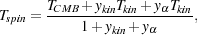
Figure 15 shows the expected global evolution of the spin temperature as a function of redshift. The blue solid line represents T_CMB, which drops as 1 + z. The green line shows the gas temperature as a function of redshift. At z 200, the gas temperature is still coupled to the CMB due to Compton scattering of the background photons off residual electrons leftover from the recombination era. At redshift ~ 200, however, the gas decouples from the CMB radiation and starts adiabatically cooling as a function of the redshift squared, (1 + z)², until the first objects start forming and heating up the gas at redshift below 30. The spin temperature (shown by the red lines) has a somewhat more complicated behavior. At z 100 it is coupled to the gas temperature due to collisional coupling caused by residual electrons leftover from recombination. At z ≈ 100 the efficiency of collisional coupling to the gas drops due to the Hubble expansion. At this stage, the spin temperature starts veering towards T_CMB until it is completely dominated by it. At lower redshifts the first astrophysical objects that heat and ionize the IGM couple T_spin to the gas. Here, broadly speaking, there are two possible histories, one in which T_spin couples to the gas as it heats up once it obtains a temperature greater than T_CMB (red solid line). In the other possible evolution the spin temperature couples to the gas much before the kinetic temperature exceeds that of the CMB (red dashed line) [8, 160, 205]. In the former case the 21 cm radiation, after decoupling from the CMB at z 30, is seen only in emission, whereas in the latter case it is seen initially in absorption and only at later stages in emission.

Figure 15. The global evolution of the CMB (blue line), gas (green line) and spin (red solid line and red dashed line) temperatures as a function of redshift. The CMB temperature evolves steadily as 1 + z whereas the gas and spin temperatures evolve in a more complicated manner (see text for detail).

Currently all attempts to measure the redshifted 21 cm emission from the IGM are focused on the redshift range 6 z 12. This is due to a number of reasons that are related to the limitations posed by the ionosphere and the background noise (see section 5 for more detail). In this range of redshifts the spin temperature is expected to be set by the astrophysics of the first objects in the Universe, namely, gas physics, feedback, etc., which often involve very complicated and poorly understood processes. However, observing the spin temperature of the Universe within the redshift window around z ≈ 50-100 will mostly probe the cosmological density field [116]. Such a measurement could provide a vast amount of information about the pristine Universe that, given the span of its redshift coverage, could potentially exceed that of the CMB data. Unfortunately however, the ionosphere at such frequencies 30 MHz poses insurmountable hurdles that render such attempts futile. This has led some authors to propose setting up radio telescopes at these very low frequencies on the moon (see e.g., [109]).

4.2. The Differential Brightness Temperature

As we mentioned above the measured quantity in radio astronomy is the brightness temperature, or more accurately the so called differential brightness temperature T_b ≡ T_b - T_CMB which reflects the fact the only meaningful brightness temperature measurement insofar as the IGM is concerned is when it deviates from T_CMB. In order to get this quantity one should substitute the various components into Equation 13. Such a substitution and rearrangement yields, [61, 62, 120, 46],

(22)

where h is the Hubble constant in units of 100 km s^-1 Mpc^-1, is the mass density contrast, x_HI is the neutral fraction, and _m and _b are the mass and baryon densities in units of the critical density. Note that the three quantities, , x_HI and T_spin, are all functions of 3D position. The term (T_spin - T_CMB) / T_spin can obtain a maximum of +1 for T_spin ≫ T_CMB, i.e., in the emission case. It has no such bound for the case of T_spin ≪ T_CMB and can be very negative in the absorption case.

Equation 22 shows that the differential brightness temperature is composed of a mixture of cosmology dependent and astrophysics dependent terms. This makes the equation a complex yet also a very informative one. This is simply because at different stages in the evolution of this field T_b is dominated by different contributions. For example, at high redshifts and before significant ionization takes place, i.e. x_HI ≈ 1, everywhere the brightness temperature is proportional to the density fluctuations making its measurement an excellent probe of cosmology. However, at low redshifts (z 7) a significant fraction of the Universe is expected to be ionized and the measurement is dominated by the contrast between the neutral and ionized regions, hence, probing the astrophysical source of ionization (see e.g., [90, 206]). Here I assumed that T_spin ≫ T_CMB at all redshifts. Figure 1, which we have discussed before, shows a typical distribution of the differential brightness temperature. The figureis taken from the simulations of Thomas et al. [206].

Most radiative transfer simulations assume that the spin temperature is much larger than the CMB temperature, namely the term (1 - T_CMB / T_spin) in eq. 22 is unity. As figure 15 shows, this is a good assumption at the later stages of reionization, however, it is probably not valid at the early stages. Modeling this effect is somewhat complex and requires radiative transfer codes that capture the Lyman- line formation and multifrequency effects, especially those coming from energetic photons [8, 129, 159, 205].

Here we show the evolution of the brightness temperature for three reionization histories: (1) With reionization, excitation and heating dominated by power law sources (miniqsos with x-rays); (2) dominated by thermal (stellar) sources; (3) dominated by a mixture of the aforementioned two types of sources. To create a contiguous observational cube or "frequency cube" (right ascension (RA) × declination (DEC) × redshift), the RA and DEC slices, taken from individual snapshots at different redshifts (or frequency), are stacked and interpolated smoothly to create a reionization history. This datacube is then convolved with the point spread function of the LOFAR telescope to simulate the mock data cube of the redshifted 21-cm signal as seen by LOFAR. For further details on creating this cube, refer to [206,

As expected, the signatures (both visually and in terms of the r.m.s) of the three scenarios (Fig. 16) are markedly different. In the miniqso-only scenario, reionization proceeds extremely quickly and the Universe is almost completely (x_HII > = 0.95) reionized by around redshift 7. The case in which stars are the only source sees reionization end at a redshift of 6. Also in this case, compared to the previous one, reionization proceeds in a rather gradual manner. The hybrid model, as explained previously, is in between the previous two scenarios.

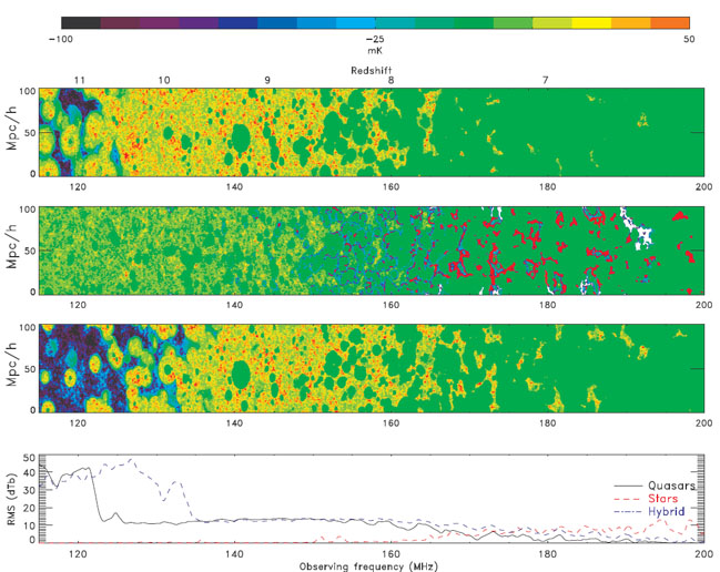Figure 16. Contrasting reionization histories: From the top, reionization histories (Tb in mK as a function of frequency or redshift) are plotted for miniqso, stellar and hybrid sources, respectively. The bottom panel plots the r.m.s of Tb as a function of redshift/frequency for all the three cases. This figure is taken from [205].

In the models shown here, the transition from the absorption dominated brightness temperature to the emission dominated one occurs at relatively low redshifts. The transition redshift depends sensitively on the assumptions made in each case. Other authors have explored such effects and conclude that the transition occurs at much higher redshifts (see e.g., the models in [129, 177]).

The T_b in Fig. 16 is calculated based on the effectiveness of the radiation flux, produced by the source, in decoupling the CMB temperature (T_CMB) from the spin temperature (T_s). This flux, both in spatial extent and amplitude, is obviously much larger in the case of miniqsos compared to that of stars, resulting in a markedly higher brightness temperature in both the miniqso-only and hybrid models when compared to that of the stars. However, we know that stars themselves produce Lyman radiation in their spectrum. Apart from providing sufficient Lyman flux to their immediate surroundings, this radiation builds up as the Universe evolves into a strong background [46], potentially filling the Universe with enough Lyman photons to couple the spin temperature to the kinetic temperature everywhere. It has to be noted that the results we are discussing here are extremely model dependent and any changes to the parameters can influence the results significantly.

4.3. The 21 cm forest at high z

Finally, I will conclude this section by discussing a very different aspect of the redshifted 21 cm radiation, and that is the case of the 21 cm forest. Very bright radio sources might exist at high redshifts. In such a case, the emission from these sources is expected to be resonantly absorbed by the neutral IGM and form a system of absorption features just like the Lyman forest seen in the spectra of distant quasars. Such absorption features are called the 21 cm forest and they were first investigated by Carilli et al. [37] and subsequently by other authors [36, 66, 64, 119, 219]. The discovery of such systems will provide very valuable information about the reionization process and the IGM's physical properties during the EoR which will be largely independent of calibration errors (see section 5). Currently, we know of no very bright high redshift sources, but with the imminent availability of highly sensitive radio telescopes like LOFAR and SKA, the prospects for detecting such sources are very promising.

Figure 17 shows a simulated spectrum at 1 kHz resolution of a z = 10 radio source with a flux density of 20 mJy at an observing frequency of 120 MHz (S₁₂₀). The implied luminosity density at a rest frame frequency of 151 MHz is then P₁₅₁ = 2.5 × 10³⁵ erg s^-1 Hz^-1. The left hand panel of Figure 17 shows a spectrum covering a large frequency range (100 MHz to 200 MHz, or HI 21cm redshifts from 13 to 6), whereas the right hand panel shows an expanded view of the frequency range corresponding to the HI 21cm line at the source redshift (129 MHz). At 129 MHz the spectrum shows a 1% drop due to the diffuse neutral IGM. See reference [37] for detail.

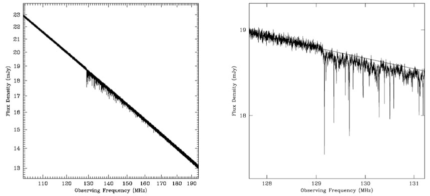Figure 17. Left hand panel: A simulated spectrum from 100 MHz to 200 MHz of a source with S120 = 20 mJy at z = 10 using the Cygnus A spectral model and assuming H I 21cm absorption by the IGM. Thermal noise has been added using the specifications of the SKA and assuming 10 days integration with 1 kHz wide spectral channels. Right hand panel: The same as the left panel, but showing an expanded view of the spectral region around the frequency corresponding to the redshift H I 21cm line at the source redshift (129 MHz). The solid line is the Cygnus A model spectrum without noise or absorption. Figure taken from [37].