


In order to reproduction the likelihoods, we need order 3 and 4 (skewness and kurtosis) terms in the multi-dimensional expansion.
In 1D, this expansion looks like:
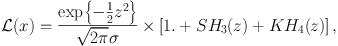 |
(29) |
where z = (x − µ) / σ, µ is the mean value and σ is the standard deviation and S and K are the skewness and kurtosis coefficients needed to adequately describe the distribution via a Hermite polynomial expansion. The skewness and kurtosis coefficients are proportional to the Markov Chain average of the respective Hermite polynomials (S∝ ⟨ H3(x) ⟩ and K∝ ⟨ H4(z) ⟩). In multiple dimensions, the simple gaussian base distribution is replaced with the fully correlated multi-dimensional gaussian:
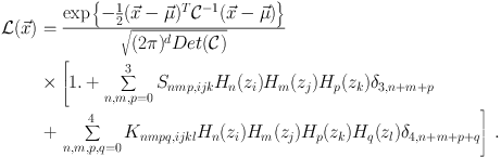 |
(30) |
Acknowledgments
It is a pleasure to thank our recent BBN collaborators Nachiketa Chakrabory, John Ellis, Doug Friedel, Athol Kemball, Lloyd Knox, Feng Luo, Marius Millea, Tijana Prodanović, Vassilis Spanos, and Gary Steigman. The work of R.H.C was supported by the National Science Foundation under Grant No. PHY-1430152 (JINA Center for the Evolution of the Elements). The work of K.A.O. was supported in part by DOE grant DE-SC0011842 at the University of Minnesota. The work of B.D.F. and T.H.Y. was partially supported by the U.S. National Science Foundation Grant PHY-1214082.