


Intrinsic alignments lead to additional contributions to the observed ellipticity correlation functions, thus compromising a simple cosmological interpretation of the results. The same is true for instrumental effects, such as contamination of the galaxy shapes by residual (uncorrected) PSF anisotropy. The impact of any systematic effect on a measurement of parameters of interest is to change the likelihood distribution for those parameters away from that which would have been observed if no systematic were present. If the systematic effect is sufficiently large, this can lead to parameter inferences that differ significantly, in a statistical sense, from the “true” values of those parameters (i.e. those that would have been found in a perfect experiment). Furthermore, the shape of the likelihood may change completely, for example from a surface with no curvature to something with significant curvature or even multi-modal features. This scenario may possibly occur in the case of intrinsic alignments, where different galaxy populations may have different intrinsic alignment signal. A joint analysis of all galaxy types could result in a multi-peaked likelihood surface in the direction of the amplitude of the intrinsic alignment effect.
Systematics can both change the measured confidence levels for a particular parameter constraint (either increasing or decreasing them) and “bias” the measurement of a parameter, that is shift the maximum likelihood away from where it would be found in the absence of the systematic. The shift in the maximum likelihood, the biasing, is a general feature of any likelihood analysis in which the incorrect model is used – in the case of intrinsic alignments either because the effect was not included or mitigated at all, or because the assumed model is not correct. The change in confidence levels, or the errors on the parameters, is more complicated and can lead to an increased sensitivity (smaller error bars), or decreased sensitivity (larger error bars) on parameters depending on the nature of the assumptions made. For example, including a model for a systematic that depends also on the parameters of interest may increase sensitivity compared to a model that does not.
The observational evidence presented in Sections 4 and 5 suggests that the amplitude of the intrinsic alignment signal is such that it will lead to significant biases in ongoing and future cosmic shear surveys. In Section 6.1 we quantify this impact for a representative cosmic shear survey. The simplest way to deal with intrinsic alignment contamination would be to measure the cosmic shear signal and then subtract the intrinsic alignment contribution (both II and GI), leaving a “pure” signal. This would require perfect knowledge of the true intrinsic alignment signal as well as total confidence in the classification of galaxies and measurement of redshifts. It is therefore not considered feasible now or in the foreseeable future. This means that it is necessary to mitigate bias from intrinsic alignments in more imaginative ways. Most of these utilise the different redshift dependences of the GG, II and GI signals, as discussed in Section 6.2. The use of “nuisance parameters” to absorb the intrinsic alignment signal is discussed in Section 6.3 and the use of auxiliary data for “self-calibration” is summarised in Section 6.4. We discuss cosmic shear three-point statistics in Section 6.5 and novel probes of the unlensed galaxy shape in Section 6.6.
The importance of intrinsic alignments for weak lensing studies was recognised early on and various studies have examined the expected impact. As early as Kamionkowski et al. (1998), novel mitigation schemes were being proposed at the same time as measurement of intrinsic alignments was being discussed.
Especially after the first detection of the cosmic shear signal (Bacon et al., 2000, Kaiser et al., 2000, Van Waerbeke et al., 2000, Wittman et al., 2000), much effort was spent on quantifying the impact of intrinsic alignments. Heavens et al. (2000) used N-body simulations to show that the impact of intrinsic alignments on cosmic shear correlation functions, as measured in their simulations, could be mitigated. They suggested that deep weak lensing surveys could be used to calibrate the importance of intrinsic alignments because the broader source redshift distribution of sources in deeper surveys reduced the relative importance of intrinsic alignments. However, this suggestion neglected the importance of GI correlations and thus cannot be relied on. Croft & Metzler (2000) also studied intrinsic alignments in N-body simulations, and whilst coming to similar conclusions as Heavens et al. (2000), the magnitude of the effect appeared to be more problematic. They suggested that the signal could be measured (calibrated) using relatively small surveys of only a few thousand galaxies at low redshift, where intrinsic alignments dominate. This signal could then be applied to wider, deeper surveys, where the shear signal could be measured. The type of observations discussed in Section 4 might be suitable for such an approach but they should not be regarded as a sufficient substitute for measurements of intrinsic alignments over the redshift range representative of the full cosmic shear survey of interest (proper coverage of galaxy types is also very important). These, and other relevant results, are discussed in more detail in Kiessling et al. (2015).
Catelan et al., (2001) considered several ways to discriminate between weak gravitational lensing and the intrinsic alignment signal. The first method that they proposed was simple, based on their particular model for intrinsic alignments, which had a strong ellipticity dependence: the impact of intrinsic alignments could be reduced by using sources with smaller intrinsic ellipticities, but this would pose serious problems for ellipticity measurement. More practically, they also suggested the use of density correlations, such as the wg+ measurements presented in this review, around galaxy clusters and the use of morphological information to remove intrinsically aligned galaxies.
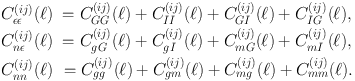
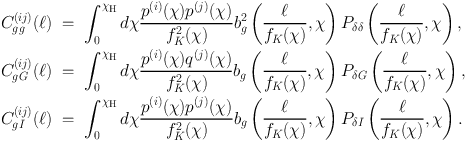
An attempt at total removal of intrinsic alignments is complicated, however, because, as we have already discussed, the observed ellipticity correlation is the sum of a gravitational lensing term, GG, an intrinsic alignment term, II, and a cross-term, GI,
 |
(33) |
where we have expressed each as a projected angular power spectrum C(ij)(ℓ) in Fourier space for a pair of tomographic bins in spherical harmonic space and ℓ denotes the angular frequency, the Fourier variable on the sky. The superscripts i, j denote a redshift bin pair for the tomographic analysis. Note that, if galaxies are well separated in redshift, any IG term is expected to be zero. The importance of the GI correlation was not fully appreciated in the earliest literature discussing mitigation (Croft & Metzler, 2000, Heavens et al., 2000, Catelan et al., 2001). This is a serious drawback as the GI term is not only more difficult to remove, it can also dominate over the II contribution for many tomographic bin pairs in realistic cosmic shear surveys. The details of the modelling of intrinsic alignments are given in our companion paper (Kiessling et al. 2015) but, for a linear alignment model, each of the 2D projected angular power spectra in Equation (33) can be constructed from the integration of the 3D power spectrum multiplied by the appropriate redshift distribution or lensing weight functions,
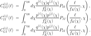 |
(34) (35) (36) |
Here fK(χ) is the comoving angular diameter distance, given by
 |
(37) |
where 1 / √|K| is interpreted as the curvature radius of the spatial part of spacetime.
p(i)(χ) = p(i)(z) dz / dχ, where p(i)(z) is the galaxy redshift distribution of bin i, q(i)(χ) is the lensing weight function of bin i (Joachimi & Bridle, 2010),
 |
(38) |
and χh is the comoving distance to the horizon. Ideally the tomographic bins do not overlap, which is possible in the case of spectroscopic redshifts. This is, however, not feasible in the case of cosmic shear surveys, which rely on photometric redshifts. Due to limitations in the precision with which photometric redshifts can be determined, as well as catastrophic outliers due to misidentification of features in the spectral energy distribution, the bins partially overlap in practice.
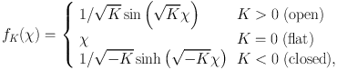
Examples of projected angular power spectra of the different GG, II, and GI terms for a projected spherical harmonic tomographic analysis of a fiducial wide-field survey are shown in Figure 13, alongside other terms related to number counts (see below). The figure shows forecasts originally made in Kirk et al. (2012). The II terms are positive (by definition), while the GI terms are negative in amplitude to match observations. Figure 13 illustrates how intrinsic alignment terms add (through the II term) and subtract (through the GI term) to the weak lensing GG power spectrum. Being a local effect, the II correlation is strongest for redshift bin auto-correlations, where the number of physically close pairs is largest. As this plot is for a photometric cosmic shear survey the redshift cross-terms do not have zero II contribution as there is usually some overlap in redshift between bins. In contrast the GI term is strongest for bins separated in redshift where the redshift distribution of the “I” bin overlaps with the lensing kernel of the “G” bin. In general the relevant weight functions overlap differently for different combinations of tomographic bins, affecting both the amplitude and effective scale dependence of each contribution to the measured shear or galaxy position correlation.
 |
Figure 13. Forecast projected angular power spectra, C(ij)(ℓ), for a tomographic analysis of a wide-field survey based on the Euclid mission design (Réfrégier et al., 2010). Upper Right Panels: Gravitational lensing and intrinsic alignment terms related to the observed ellipticity auto-correlation (GG, GI, II) and galaxy clustering and cosmic magnification terms related to the number count auto-correlation (gg, gm, mm). Lower Left: Terms related to the cross-correlation of ellipticity and number counts, including contributions from intrinsic alignment and magnification (gG, mG, gI, mI). The absolute value of these power spectra are shown but it should be remembered that the GI, gI and mI contributions are negative in amplitude. See Section 6.4 for more details on these power spectra. The numbers in the top right corner of each panel denote the tomographic bin pair being considered. There are 10 bins in total, split so each has roughly the same number density of source galaxies; bin 1 is the lowest redshift bin, while bin 10 is the highest redshift bin. See Sections 6.1 and 6.4for detailed descriptions of each term. Reproduced with permission from Kirk et al. (2012). |
Some features of the impact of intrinsic alignments on two-point statistics, as well as simple mitigation techniques, are brought together in Figure 14. Here we forecast constraints on cosmology from a generic weak gravitational lensing survey, modelled on the European Space Agency Euclid mission 8 (Réfrégier et al., 2010, Laureijs et al., 2011). This generic survey covers 15,000 deg2 with a galaxy density of 30 arcmin−2, split into 10 tomographic redshift bins over the range 0 < z < 2.0. A Gaussian total shape noise contribution of σє = 0.35 is assumed. Our results are shown as 95% confidence contours in the dark energy equation of state parameters w0 and wa. These describe the amplitude and time-evolution of the dark energy equation of state, wde(z) = w0 + wa(1−a). All constraints are shown marginalised over the cosmological parameters: Ωm, the dimensionless matter density, Ωb, the dimensionless baryon density, σ8, the amplitude of the density perturbations, h, the Hubble parameter, and ns, the spectral index of the density perturbations. Euclid is an example of a Stage-IV survey as defined by the Dark Energy Task Force (Albrecht et al., 2006).
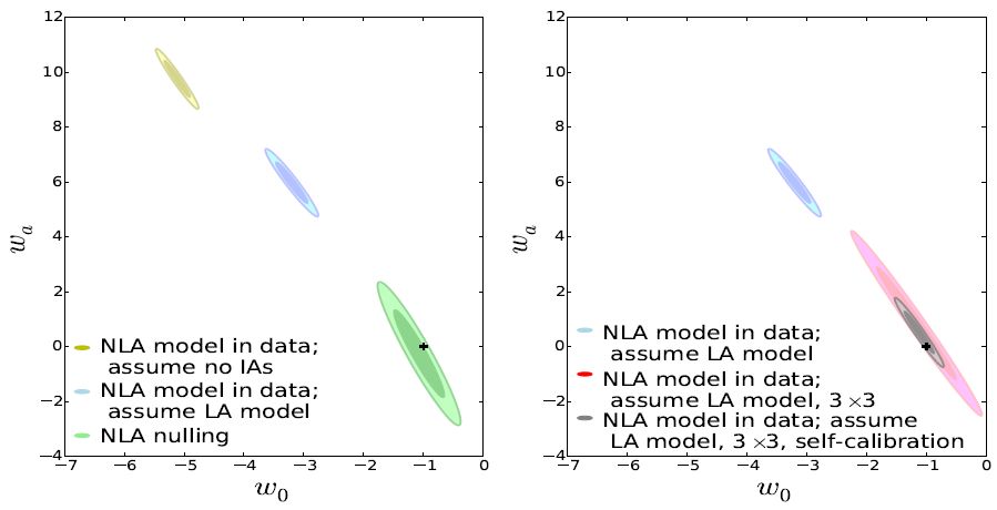 |
Figure 14. Forecast cosmological constraints for a generic Euclid-like survey, making different assumptions about intrinsic alignments. 95% confidence ellipses are shown for the dark energy equation of state parameters, w0 and wa. Constraints shown have been marginalised over Ωm, h, σ8, Ωb, ns and nuisance parameters where appropriate, see Section 6.1 for more details. Left Panel: Impact of incorrect model choice. True model assumed is the non-linear alignment model (Hirata & Seljak, 2004, Bridle & King, 2007). The yellow contour shows constraints and bias on w0, wa when intrinsic alignments are ignored. The blue contour assumes the (incorrect) linear alignment model. The green contour shows the constraints from nulling, see Section 6.2 for more details. Right Panel: Impact of marginalising over a robust grid of nuisance parameters in redshift and angular scale and self-calibration with galaxy clustering information. Each contour uses the non-linear alignment model as the “truth”. The blue contour is the same as in the left-hand panel i.e. it assumes the (incorrect) linear alignment model. The red contour also assumes the linear alignment model, marginalised over a 3 × 3 grid of nuisance parameters in redshift and angular scale. The grey contour shows the same scenario (assume linear alignment, 3 × 3 nuisance grid) with the inclusion of galaxy clustering information i.e. self-calibration, see Section 6.4 for more details. The black crosses show the fiducial values of w0, wa. |
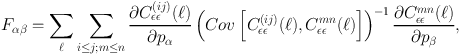
The constraints are calculated by the Fisher matrix technique (Fisher, 1935), assuming a Gaussian likelihood function and covariance matrix, independent of the fiducial cosmological parameter values. The Fisher matrix approach can be extended to make an estimate of the bias on cosmological parameters, Δ pα, when an incorrect cosmological model is assumed (Huterer et al. 2006; see also Amara & Réfrégier 2008 and Appendix A of Joachimi et al. 2011):
 |
(39) |
where Δ Cєє(ij)(ℓ) is the difference between the power spectra for the true and assumed models; F is the Fisher matrix,
 |
(40) |
Cov is the covariance matrix (Takada & Jain, 2004); i, j, m, n count over tomographic redshift bins and α,β count over some set of cosmological (and nuisance) parameters. pα refers to a particular cosmological or nuisance parameter, hence Δ pα is the resulting bias on that parameter. The equations refer to the ellipticity-ellipticity auto-correlation, Cєє(ij) (ℓ), and the bin pairs are restricted to i ≤ j because the symmetry of the observable means that these pairs exhaust the available information. The formalism is easily extendable to the galaxy position-position correlation, Cnn(ij) (ℓ), and the position-ellipticity cross-term, Cnє(ij) (ℓ), see Section 6.4 below for more details.
We can use this to show the importance of a well-modelled intrinsic alignment contribution to the measured cosmic shear signal. We do not know the true intrinsic alignment model but the left-hand panel of Figure 14 shows the bias on cosmological parameters when we take the non-linear alignment model (with an amplitude of C1 = 5 × 10⁻¹⁴(h2 M⊙ Mpc−3)−1 (Bridle & King, 2007) and, for simplicity, no dependence on galaxy type or luminosity) as the (true) observed signal but use either no intrinsic alignments (yellow contour) or the linear alignment model (blue contour) in our analysis. The assumed intrinsic alignment amplitude is based on the SuperCOSMOS normalisation (Brown et al., 2002, Bridle & King, 2007) and is consistent with the lower end of current observational constraints for early-type galaxies (Joachimi et al., 2011, Heymans et al., 2013), making the bias predictions realistic for current and future cosmic shear surveys. It is clear that the results are catastrophically biased. The true fiducial cosmology is indicated by a black cross and the forecast contours are off by several standard deviations. The contour that assumes the linear alignment model (blue) is less biased than that which ignores intrinsic alignments completely because the linear alignment model replicates the non-linear alignment phenomenology at linear scales.
Cosmic shear in tomographic redshift slices is an approximation of a more general formalism called 3D cosmic shear, the most notable being the Limber approximation, a binning in redshift. 3D cosmic shear uses the one-point shear transform coefficients that are calculated using a spherical-Bessel transform of the data (Heavens, 2003). The impact and mitigation of intrinsic alignments in 3D cosmic shear analysis has been studied in Kitching et al. (2008), Merkel & Schäfer (2013), Kitching et al. (2014b), Kitching et al. (2014a). Results and strategies presented below are framed for tomographic analyses but can in principle also be applied to the 3D cosmic shear methodology.
6.2. Exploiting redshift dependence
Taking a conservative approach, one can assume a complete lack of knowledge about the physics underlying intrinsic alignments and thus the form of the II and GI spectra. In that case the only reliable information left to separate the weak lensing signal from intrinsic alignments is the redshift dependence of the signals, which is governed by the redshift distribution of the galaxy samples and their lensing weight functions (see Equations (34) to (35)). Here we describe some appraoches which exploit this information:
Downweighting: King & Schneider (2002) proposed an algorithm to suppress the II term in non-tomographic weak lensing surveys with photometric redshift information. They demonstrated that incorporating a Gaussian kernel that downweights galaxy pairs close in redshift is effective at reducing the intrinsic alignment contamination while moderately reducing the effective number of galaxies in the analysis. In a similar analysis Heymans & Heavens (2003) derived statistically optimal weights for suppressing the II term if either photometric or spectroscopic redshift information is available. They concluded that high-quality photometric redshifts would be a necessity for the analysis of future weak lensing surveys.
Using redshifts to divide the galaxy sample into tomographic bins, King & Schneider (2003) fitted a linear combination of generic template functions to II and GG correlation functions. If the redshift overlap of neighbouring tomographic bins is small, it may well be sufficient to simply discard all redshift auto-correlations from analysis, which causes a 10 % increase in errors on cosmological parameters when at least five tomographic bins are used (Takada & White, 2004). This approach was extended to include the GI term by King (2005), assuming independence of the II and GI terms, and demonstrated on toy models.
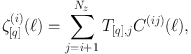
Nulling: Joachimi & Schneider (2008, 2009) introduced a nulling technique for the GI term. For a given set of tomographic two-point statistics in Nz tomographic bins, one can construct new measures, the nulled power spectrum ζ, via linear combinations of the standard statistics, e.g. in the case of projected angular power spectra,
 |
(41) |
with weights T[q], j, for every foreground redshift bin i. The weights are orthogonal to each other, and orthogonal to 1 − χ(zi) / χ(zj), which is an approximation to the kernel of the GI term in the limit of redshift bins with narrow redshift distributions; compare to Equation (36). Depending on implementation, the redshifts zi and zj can correspond to the mean or median redshifts in each tomographic bin. In this way one can construct Nz − i − 1 independent statistics ζ[q](i) for every foreground bin, numbered by the index q in square brackets, in which the intrinsic alignment signal should be strongly suppressed.
Joachimi & Schneider (2008) showed that nulling, combined with a suppression of redshift auto-correlations, reduces the bias due to the combination of II and GI by at least an order of magnitude on well-constrained cosmological parameters. This was achieved robustly over a wide range of photometric redshift parameters, for random scatters up to 0.1(1 + z) and catastrophic outlier (galaxies whose redshifts are comprehensively misidentified) fractions up to 10 %. However, due to the similar redshift scaling of the GI and GG signals, the robust removal of GI contamination comes at the price of substantially reducing the statistical power. Marginal errors on cosmological parameters increase by typically a factor of two, and by a factor of three in case of the dark energy equation of state parameters w0 and wa, whose constraints rely strongly on the redshift evolution of the lensing signal. While an order of magnitude loss in the dark energy figure of merit is intolerable for cosmological surveys, nulling techniques and their kin can still serve as a robust validation test for intrinsic alignment mitigation strategies that rely on more assumptions about the nature of these signals.
We show schematically the power of nulling in the left panel of Figure 14. The green contour shows the results of a nulling analysis of the same experimental scenario as for the other contours. Nulling succesfully reduces the bias to within the 1σ contour but at the cost of reducing usable information, hence the ellipse is broader i.e. less constraining.
Boosting: As was already noted in the early works (e.g. King & Schneider, 2002, King & Schneider, 2003), any procedure to suppress the intrinsic alignment contribution can be reversed to boost these signals, which enables their study at scales and redshifts where the lensing signal would otherwise dominate. Joachimi & Schneider (2010) devised a GI boosting technique, again via linear combinations of tomographic two-point statistics and showed explicitly how it links to nulling. The method can turn a GI signal that is 10−30 % of the GG term into being about one order of magnitude stronger than GG for good quality photometric redshifts and two orders of magnitude stronger for spectroscopic redshifts. Recently, Schneider (2014) refined this concept to boost the galaxy-magnification cross-correlation over the galaxy clustering signal, which de-biased and tightened cosmological constraints.
6.3. Parameterisation and marginalisation
The most common approach to dealing with intrinsic alignments in the literature is to introduce a number of free parameters that describe the amplitude, redshift/scale/colour dependence etc. of intrinsic alignments and allow these parameters to vary within some prior range as part of a cosmological likelihood analysis. These intrinsic alignment “nuisance” parameters can be marginalised over when quoting constraints on cosmological parameters. This marginalisation will make cosmological parameter constraints weaker but, if the nuisance parameterisation is sufficiently flexible that it captures the full range of the intrinsic alignment signal, the resulting constraints will be unbiased. Note that the model being parameterised can be based on an assumed physical mechanism for intrinsic alignments and is therefore not distinct from the linear alignment or non-linear alignment models discussed above. For example Heymans et al. (2013) uses the non-linear alignment model with a single free amplitude parameter, which is marginalised over whenever constraints on cosmological parameters are discussed. See Section 4.3 for a more detailed discussion.
The benefit of the parameterisation/marginalisation approach is that it can be implemented simultaneously with the cosmological parameter estimation. This means that the same procedure produces constraints on cosmological parameters and the parameters of the intrinsic alignment model. The downside is that a higher dimensional parameter space must be explored, sometimes significantly higher, which is computationally expensive. There is also some ambiguity in the statement that cosmological constraints are unbiased “provided the parameterisation is sufficiently flexible.” In the absence of very strong constraints on intrinsic alignments there is no definitive statement about either how many nuisance parameters are required or what their prior ranges should be. With this approach, it is easy to update the analysis as more precise measurements of intrinsic alignments become available, either through a joint likelihood analysis or by altering the priors of the initial analysis.
In the right-hand panel of Figure 14 we show an attempt to reduce bias through nuisance parameters and marginalisation for our toy survey. We also show the use of self-calibration to recover information through full exploitation of joint gravitational shear and galaxy position information, described in Section 6.4 below. Each contour takes the non-linear alignment model to be the true description of intrinsic alignments but models them (incorrectly) with the linear alignment model. The blue contour is the same as in the left hand panel, showing the bias this produces in the simple case.
The red contour is the result of the same analysis with additional nuisance parameters included. A grid of nuisance parameters which can vary in scale and redshift is employed: 3 × 3 parameters in z × k, where k is the Fourier space wavenumber, are used for both the amplitude of the II and GI terms, as well as free amplitudes for each. This leads to a total of 2(3 × 3) + 2 = 20 nuisance parameters. Marginalising over these new parameters reduces the precision, as shown by the increased size of the contour, but it also reduces the bias in the inferred cosmological parameters to within the 1σ area. For a more detailed example of marginalisation using this parameterisation see Joachimi & Bridle (2010).
A goal of the parameterisation and marginalisation approach is to include information from intrinsic alignment measurements as physically motivated priors on the intrinsic alignment nuisance parameters. This inclusion of prior information from observations is not yet mature in the intrinsic alignment literature but, for example, Sifón et al. (2015) used measurements of intrinsic alignments in clusters to inform parameters for their implementation of the halo model. They aimed to test how strong a deviation from the non-linear alignment model at small scales was allowed by observations. They found an allowed deviation significantly lower than the fiducial model assumed in Schneider & Bridle (2010).
All cosmic shear surveys contain information beyond the correlation of galaxy ellipticities. Even a survey with photometric-quality redshifts can be used to study galaxy clustering (i.e. position-position correlations), and additional information is contained in the cross-correlation between position and ellipticity. Exploitation of this additional information can regain some of the constraining power lost when marginalising over intrinsic alignment nuisance parameters. Bernstein (2009) outlined the formalism to treat a range of two-point correlations available with cosmic shear survey data. We summarise relevant aspects below and refer readers to that paper for more details.
Exploitation of this information is an example of “self-calibration” because the uncertainties due to intrinsic alignments are being calibrated by information contained in the cosmic shear survey itself. The effect of magnification is important in both galaxy position-galaxy position clustering and the galaxy position-ellipticity cross-correlation, so omitting it can bias results (Duncan et al., 2014). We can now write down a set of three observables, each made up of multiple contributions, analogous to Equation (33),
 |
(42) (43) (44) |
These are the set of power spectra shown in Figure 13. As before “G” denotes gravitational lensing and “I” intrinsic alignment, we use “g” and “m” to refer to galaxy clustering and the change in number density due to magnification respectively (see below for more details). єє is then the observed ellipticity correlation signal from both weak lensing and intrinsic alignment contributions while nn is the observed galaxy position correlation signal including the magnification contributions. nє is the observed cross-correlation.
The gG term is the cross-correlation of galaxy clustering and gravitational lensing. As galaxies are biased tracers of the underlying matter distribution, we would expect a foreground galaxy population to be correlated with the lensing of background source galaxies. This is often referred to as galaxy-galaxy lensing, especially on scales where the lensing is dominated by the haloes of the foreground galaxies (e.g. Mandelbaum et al., 2006b, van Uitert et al., 2011, Velander et al., 2014). It is clear that a galaxy-intrinsic alignment term, gI, appears in the galaxy-shear cross-correlation in an analogous way to the gravitational lensing-intrinsic alignment GI term. Consequently, intrinsic alignments are an important contamination in galaxy-galaxy lensing if the source and lens populations cannot be perfectly separated (Blazek et al., 2012, Chisari et al., 2014). We can write the projected angular power spectra of these terms as integrals over the three dimensional matter power spectrum and the appropriate window functions under the Limber approximation:
 |
(45) (46) (47) |
Weak gravitational lensing, as well as distorting the shape of galaxy images, changes their apparent sizes while the surface brightness is unchanged. This means that the flux of galaxies is changed and galaxy images can be either magnified or demagnified. This is the cosmic magnification contribution referred to by the subscript m. For a flux-limited survey this can mean galaxies are promoted or demoted across the detection threshold, changing the observed number density and the clustering statistics. Magnification also causes a change in effective area, which also modulates the observed number density. This is apparent in the mm term that contributes to the observed galaxy correlation, but there are also cross-correlations between magnification and galaxy counts, gm, mg, and cross-correlations between magnification and gravitational lensing, mG, and indeed, magnification-intrinsic alignment correlations, mI.
Magnification due to lensing arises due to the same gravitational potential responsible for the shear, therefore the magnification signal can be related to the correlation functions that involve the shear. The amplitude of the effect depends on α(i), the power-law slope of the observed number counts for the galaxies in the ith tomographic bin. The form of the magnification terms is
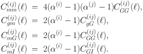 |
(48) (49) (50) (51) |
These magnification terms are important because results from an analysis that ignores them can be significantly biased (Duncan et al., 2014).
Exploitation of some of this set of observables has been proposed in different ways (Zhang, 2010, Troxel & Ishak, 2012b, Troxel & Ishak, 2012a) and has been shown to be an effective self-calibration strategy in forecasts (Bernstein, 2009, Joachimi & Bridle, 2010, Laszlo et al., 2012, Kirk et al., 2013). Even if intrinsic alignment model ignorance is aggressively marginalised over, self-calibration can recover the bulk of the information present in a naive cosmic shear analysis that ignored intrinsic alignments, but without the bias on cosmology. This approach has yet to be attempted as part of a real data analysis because the statistical power of existing datasets does not warrant such a thorough treatment.
An example of the power of this self-calibration approach is shown in
the forecasts of Figure 14. We have already
shown how marginalisation over nuisance parameters can remove the
cosmological bias due to intrinsic alignments, at the cost of
constraining power. The grey contour in the right-hand panel uses the
same approach but includes galaxy clustering information and galaxy +
weak gravitational lensing cross-correlation, all from the same
(photometric) survey as the cosmic shear
signal. In the case where multiple probes are considered we replace the
simple C(ij)(ℓ) with a data vector, for
example  (k) =
{Cєє(ij) (ℓ),
Cnє(ij) (ℓ),
Cnn(ij) (ℓ)}, where k
counts over bin pairs. Note that the inclusion of the
Cnє(ij) (ℓ)
cross-correlations breaks the bin pair symmetry and each bin pair
i, j must be considered separately. The same grid
parameterisation is extended to galaxy bias and the galaxy + weak
gravitational lensing cross-correlation amplitude, giving an extra 20
nuisance parameters for a total of 40. Even with these new nuisance
parameters, the self-calibration result is much tighter than that of
weak gravitational lensing alone while remaining unbiased at 1
σ. Indeed the self-calibration with 40 nuisance parameters is on
a par with the naive weak gravitational lensing
analysis without nuisance parameters in terms of constraining power.
(k) =
{Cєє(ij) (ℓ),
Cnє(ij) (ℓ),
Cnn(ij) (ℓ)}, where k
counts over bin pairs. Note that the inclusion of the
Cnє(ij) (ℓ)
cross-correlations breaks the bin pair symmetry and each bin pair
i, j must be considered separately. The same grid
parameterisation is extended to galaxy bias and the galaxy + weak
gravitational lensing cross-correlation amplitude, giving an extra 20
nuisance parameters for a total of 40. Even with these new nuisance
parameters, the self-calibration result is much tighter than that of
weak gravitational lensing alone while remaining unbiased at 1
σ. Indeed the self-calibration with 40 nuisance parameters is on
a par with the naive weak gravitational lensing
analysis without nuisance parameters in terms of constraining power.
Similarly, it has been shown that information contained in changes to the size of lensed galaxy images due to magnification can be exploited in parallel with that from image shape distortion (Heavens et al., 2013, Alsing et al., 2014). Using this magnification information mitigates the impact of intrinsic alignments by ∼ 20%, even in a pessimistic scenario. This information can also be included as part of a general self-calibration scheme, along with galaxy clustering information.
Self-calibration exploits information beyond shape measurements present in any cosmic shear survey. It is of course possible to calibrate uncertainty, from intrinsic alignments or other sources, by utilising additional data from beyond the optical weak lensing survey in question. This could mean assuming priors on cosmological parameters from cosmic microwave background (CMB) experiments, the use of spectroscopic redshift surveys to calibrate photometric redshift estimates or cross-correlation with a different dataset. The potential for measuring galaxy shapes in radio surveys has been noted (Brown et al., 2015). This could be used to make a weak lensing measurement in the radio or to calibrate shape measurement systematics or the intrinsic alignment signal in an optical weak lensing survey (Kitching et al., 2015, Kirk et al., 2015, Patel et al., 2015). A note of caution should be drawn from Patel et al. (2010) however, who found no evidence of correlation between shapes measured in optical and radio surveys. Further work is required to determine the true relationship between galaxy shapes in optical and radio wavelengths. If they were truly uncorrelated, they could not be used for mutual calibration but the effective number density of the combined surveys would be increased by a factor of two. We discuss novel approaches to intrinsic alignment mitigation using radio surveys in Section 6.6 below.
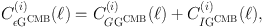
Another interesting cross-correlation is between weak lensing of galaxy images and weak lensing of the CMB (Hand et al., 2015, Troxel & Ishak, 2014, Hall & Taylor, 2014). Light from the CMB is lensed on its way to the observer, just like light from galaxies. In the case of the CMB there is a single source plane, the surface of last scattering, and the light pattern contains the imprinted signal of all the structure formation from last scattering until today. There is no equivalent to intrinsic alignments in the source of the CMB. However, when one cross-correlates the weak gravitational lensing signal from galaxies with that from the CMB, which we indicate by єGCMB, there will also be a cross-term from galaxy intrinsic alignments and the CMB lensing:
 |
(52) |
where i labels a weak gravitational lensing tomographic bin (the CMB lensing has only one source plane). The contribution of this term to the observed cross-correlation signal has been estimated to be ∼ 15% (Hall & Taylor, 2014) in a survey combination such as the ACTPol/CFHT (Atacama Cosmology Telescope-polarisation/Canada France Hawaii Telescope) Stripe 82 cross-correlation of Hand et al. (2015). Troxel & Ishak (2014) suggested a self-calibration technique for the CMB-intrinsic alignment correlation using a scaling relation between the intrinsic alignment information in the weak gravitational lensing and the combined weak gravitational lensing and CMB observables. They claim that this self-calibration allows one to reduce the impact of intrinsic alignments in the cross-correlation by a factor of 20 or more in all redshift bins.
6.5. Higher-order cosmic shear statistics
The three-point statistics of the shear field can in principle be used to mitigate the intrinsic alignment systematics in the two-point analysis, because the dependencies of the three-point intrinsic alignment terms on cosmological parameters is different from those in the two-point measurement (Vafaei et al., 2010). In the three-point case, the correlation terms that arise have the form GGG, IGG, GII and III (and combinatorial variations thereof). The origin is analogous to that of two-point intrinsic alignments; here GGG is the pure gravitational lensing three-point, IGG contains one intrinsic alignment term, GII contains two and III is the three-point intrinsic alignment auto-correlation.
The most recent observations of three-point cosmic shear were presented in Fu et al., (2014). They inferred constraints on three-point intrinsic alignments by including it in their mode and found a slight improvement in cosmological parameter measurements when intrinsic alignments were included. The amplitude of the three-point intrinsic alignment signal was tested using simulations in Semboloni et al., (2011), who found that third-order weak lensing statistics are typically more strongly contaminated by intrinsic alignments than second-order shear measurements, which leads to the possibility of using three-point statistics to measure the intrinsic alignment amplitude and constrain intrinsic alignment models. This knowledge of intrinsic alignments could then be used to improve the accuracy of two-point cosmic shear measurements. Shi et al., (2010) applied the nulling method to three-point statistics and showed that a factor of ten suppression can be achieved in the GGI/GGG ratio. Valageas, (2014) found that source-lens clustering can affect both two- and three-point statistics, and that the intrinsic alignment bias is typically about 10% of the signal for both two-point and three-point statistics.
Higher than second-order statistics are essential to studies of non-Gaussianity in the weak lensing signal. One way to access the full information encoded in weak lensing is to produce reconstructed maps of convergence or mass (Kaiser & Squires, 1993) from cosmic shear surveys. These maps can then be analysed statistically, for example the counting of peaks in the convergence distribution is a source of cosmological information (e.g. Bacon & Taylor, 2003, Van Waerbeke et al., 2013). Pires et al. (2012) showed that these peak counts capture rich non-Gaussian information beyond the skewness and kurtosis of the distribution, while Dietrich & Hartlap (2010) showed significant statistical improvement when peak counts were combined with two-point statistics. Alternatively, topological features can be exploited by decomposing the map into Minkowksi functionals (Kratochvil et al., 2012, Petri et al., 2013, Shirasaki & Yoshida, 2014). The impact of intrinsic alignments on mass reconstruction, peak counts and Minkowski functionals is a subject of current study. Simon et al. (2009) included intrinsic alignments in their mass reconstruction estimator, based on 3D cosmic shear, while a new peak counts model has been proposed by Lin & Kilbinger (2015) which can be adapted to include intrinsic alignments.
6.6. Probes of the unlensed galaxy shape
One potentially very useful avenue for the control of intrinsic alignments is the use of observables that can access information about the intrinsic (or “unlensed”) galaxy shapes and/or orientations. Here we discuss two possible observables of this type: the polarised emission from background galaxies observed in the radio (Section 6.6.1) and estimates of the rotation velocity axis of disc galaxies (Section 6.6.2).
6.6.1. Radio polarisation as a tracer of intrinsic orientation
Several authors have demonstrated from a theoretical perspective that, for observations using radio telescopy, the local plane of polarisation is not altered by gravitational light deflection effects (Kronberg et al., 1991, yer & Shaver, 1992, Faraoni, 1993, Surpi & Harari, 1999). This property was first exploited by Kronberg et al., [1991, who developed and applied a technique for measuring gravitational lensing using polarisation observations of the resolved radio jets of distant quasars.
Audit & Simmons, (1999) demonstrated how the integrated polarisation emission from “normal” star-forming galaxies could in principle be included in weak lensing estimators of the parameters describing intervening lenses. The fundamental assumption underlying the technique is that the orientation of the integrated polarised emission from a background galaxy is a noisy tracer of the intrinsic structural position angle of the galaxy. Kronberg et al., (1991) and Audit & Simmons, (1999) focused on the reduction in uncertainty on estimates of the lensing shear signal that is afforded by including the polarisation information.
It was further shown in Brown & Battye, (2011) that the use of polarisation may potentially be a powerful tool to help separate intrinsic alignments from weak lensing distortions of galaxy shapes. The idea is that optical surveys provide a measure of the intrinsic ellipticity plus the shear from weak lensing, while the radio polarisation provides information about the unlensed galaxy orientation. In combination, these estimators effectively provide a measure of the difference between the intrinsic and observed orientations of individual galaxies. They are by construction insensitive to contamination by intrinsic alignments in the limit of a perfect relationship between the orientation of the polarised emission and the structural position angle. The weak lensing analysis could be conducted using radio images alone (Brown et al., 2015) but this type of measurement has been limited to date by the low source counts available (Chang et al., 2004).
Figure 15 shows an apparent alignment between polarisation pseudo-vectors and total intensity from radio wavelengths (Berkhuijsen et al., 2003) for the galaxy M31. Stil et al. (2009) further suggested alignment between the polarisation orientation and the emission at optical wavelengths. If this relationship was found to generally hold, one could potentially use the radio polarisation orientation as a proxy for the optical intrinsic position angle in order to mitigate intrinsic alignments in overlapping optical and radio surveys. However in order to fully exploit this potential, in addition to understanding the relationship between polarisation and structural position angles, one would also require a much deeper understanding of the correlation between the shapes of galaxies as measured in optical data and their shapes as measured from radio observations. At the current time, the situation with respect to this issue is not clear and more work is required in advance of results from the SKA, Euclid and LSST (Patel et al., 2010, Brown et al., 2015, Patel et al., 2015). One benefit of shape measurements from both radio and optical surveys is that shape measurement systematics are expected to be very different for each, so cross-correlation of measured shapes should reduce the impact of these measurement systematics (Bacon et al., 2015).
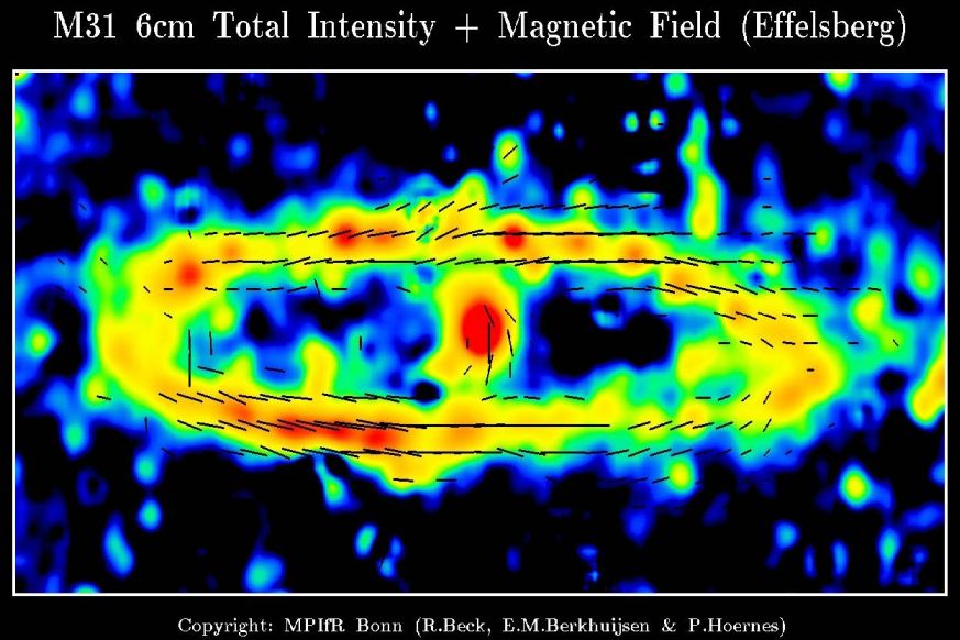 |
Figure 15. Total emission (colour scale) and polarised emission (black vectors) from M31 at λ = 6.2 cm, smoothed to an angular resolution of 5 arcmin. Contour levels are 5, 10, 15, 20, 30, 40 and 60 mJy/beam area. Reproduced with permission from ??? © ESO. |
6.6.2. Rotational velocities as a tracer of intrinsic orientation
A second novel approach is to use rotational velocity measurements to provide information about the intrinsic shapes of galaxies. The idea, first suggested by Blain, (2002) and Morales, (2006), is to measure the axis of rotation of a disc galaxy and to compare this to the orientation of the major axis of the galaxy disc image. In the absence of lensing, these two orientations should be perpendicular, so measuring the departure from perpendicularity directly estimates the shear field at the galaxy's position. The basic technique is illustrated in Figure 16.
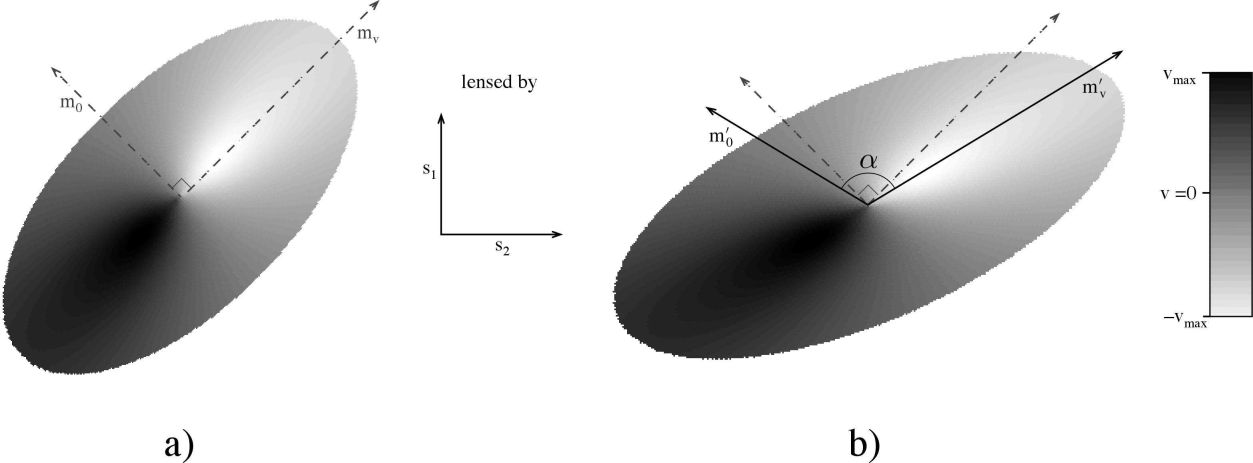 |
Figure 16. An illustration of the rotational velocity lensing technique. The grey scale indicates the observed radial velocity. A model galaxy in the absence of lensing is shown in the left-hand panel, where the zero velocity axis (m0) and the axis defined by the maximum radial velocity (mv) are perpendicular. The application of a shear (here applied along the s1 and s2 axes) breaks this perpendicularity. The observed angle α directly measures the shear component. © AAS. Reproduced with permission from Morales (2006). |
We note that this technique can in principle be applied in both the radio and optical bands, making use of spectral line observations in the former and spectroscopic observations in the latter. It is worth pointing out that many future radio surveys plan to conduct HI line observations alongside continuum-mode observations (which can be done at no extra cost in terms of telescope time).
The rotation velocity technique shares many of the characteristics of the polarisation approach described above – in the limit of perfectly well-behaved, infinitely thin disc galaxies, it is also free of shape noise and it can also be used to remove the contaminating effect of intrinsic galaxy alignments. In practice, the degree to which the rotational velocity technique improves on standard methods will be dependent on observational parameters. First, one would need to account for the fact that the HI line emission of galaxies is much fainter than the broad-band continuum emission and so the number of galaxies will be reduced. Secondly, for a population of real disc galaxies, there will again be some scatter in the relationship between the rotation axis and the major axis of the galaxy disc. Recently Huff et al., (2013) proposed to extend this technique using the Tully-Fisher relation to calibrate the rotational velocity shear measurements and thus reduce the residual shape noise even further. This approach would require overlapping photometric and spectroscopic survey data.
8 http://www.euclid-ec.org/ Back.