Copyright © 1999 by Annual Reviews. All rights reserved
| Annu. Rev. Astron. Astrophys. 1999. 37:311-362
Copyright © 1999 by Annual Reviews. All rights reserved |


The most fundamental fact about molecular clouds is that most of their
contents are invisible. Neither the H2 nor the He in the bulk
of the clouds are excited sufficiently to emit. While fluorescent
emission from H2 can be mapped over the face of clouds
(Luhman & Jaffe 1996),
the ultraviolet radiation
needed to excite this emission does not penetrate the bulk of the cloud.
In shocked regions, H2 emits rovibrational lines that are
useful probes of TK and
 (
( ) (e.g.
Draine & McKee 1993).
Absorption by H2 of background stars is also difficult: the
dust in
molecular clouds obnubilates the ultraviolet that would reveal electronic
transitions; the rotational transitions are so weak that only huge N
would produce absorption, and the dust again obnubilates background sources;
only the vibrational transitions in the near-infrared have been seen
in absorption in only a few molecular clouds
(Lacy et al 1994).
Gamma rays resulting from cosmic ray interactions with atomic nuclei do
probe all the material in molecular clouds
(Bloemen 1989,
Strong et al 1994).
So far, gamma-ray studies have suffered from low spatial resolution
and uncertainties in the cosmic ray flux; they have been used mostly to
check consistency with other tracers on large scales.
) (e.g.
Draine & McKee 1993).
Absorption by H2 of background stars is also difficult: the
dust in
molecular clouds obnubilates the ultraviolet that would reveal electronic
transitions; the rotational transitions are so weak that only huge N
would produce absorption, and the dust again obnubilates background sources;
only the vibrational transitions in the near-infrared have been seen
in absorption in only a few molecular clouds
(Lacy et al 1994).
Gamma rays resulting from cosmic ray interactions with atomic nuclei do
probe all the material in molecular clouds
(Bloemen 1989,
Strong et al 1994).
So far, gamma-ray studies have suffered from low spatial resolution
and uncertainties in the cosmic ray flux; they have been used mostly to
check consistency with other tracers on large scales.
In the following subsections, I will discuss probes of different physical quantities, including some general results, concluding with a discussion of the observational and analytical tools. Genzel (1992) has presented a detailed discussion of probes of physical conditions.
3.1. Tracers of Column Density, Size, and Mass
Given the reticence of the bulk of the H2, essentially all probes of physical conditions rely on trace constituents, such as dust particles and molecules other than H2. Dust particles (Mathis 1990, Pendleton & Tielens 1997) attenuate light at short wavelengths (ultraviolet to near-infrared) and emit at longer wavelengths (far-infrared to millimeter). Assuming that the ratio of dust extinction at a fixed wavelength to gas column density is constant, one can use extinction to map N in molecular clouds, and early work at visible wavelengths revealed locations and sizes of many molecular clouds before they were known to contain molecules (Barnard 1927, Bok & Reilly 1947, Lynds 1962). There have been more recent surveys for small clouds (Clemens & Barvainis 1988) and for clouds at high latitude (Blitz et al 1984). More recently, near-infrared surveys have been used to probe much more deeply; in particular, the H−K color excess can trace N to an equivalent visual extinction, Av ∼ 30 mag (Lada et al 1994, Alves et al 1998a). This method provides many pencil beam measurements through a cloud toward background stars. The very high resolution, but very undersampled, data require careful analysis but can reveal information on mass, large-scale structure in N and unresolved structure (Alves et al 1998a). Padoan et al (1997) interpret the data of Lada et al (1994) in terms of a lognormal distribution of density, but Lada et al (1999) show that a cylinder with a density gradient, n(r) ∝ r−2, also matches the observations.
Continuum emission from dust at long wavelengths is complementary to absorption studies (e.g. Chandler & Sargent 1997). Because the dust opacity decreases with increasing wavelength (κ(ν) ∝ νβ, with β ∼ 1−2), emission at long wavelengths can trace large column densities and provide independent mass estimates (Hildebrand 1983). The data can be fully sampled and have reasonably high resolution. The dust emission depends on the dust temperature (TD), linearly if the observations are firmly in the Rayleigh-Jeans limit, but exponentially on the Wien side of the blackbody curve. Observations on both sides of the emission peak can constrain TD. Opacities have been calculated for a variety of scenarios including grain mantle formation and collisional concrescence (e.g. Ossenkopf & Henning 1994). For grain sizes much less than the wavelength, β ∼ 2 is expected from simple grain models, but observations of dense regions often indicate lower values. By observing at a sufficiently long wavelength, one can trace N to very high values. Recent results indicate that τD(1.2 mm) = 1 only for Av ∼ 4 × 10⁴ mag (Kramer et al 1998a) in the less dense regions of molecular clouds. In dense regions, there is considerable evidence for increased grain opacity at long wavelengths (Zhou et al 1990, van der Tak et al 1999), suggesting grain growth through collisional concrescence in addition to the formation of icy mantles. Further growth of grains in disks is also likely (Chandler & Sargent 1997).
The other choice is to use a trace constituent of the gas, typically molecules that emit in their rotational transitions at millimeter or submillimeter wavelengths. By using the appropriate transitions of the appropriate molecule, one can tune the probe to study the physical quantity of interest and the target region along the line of sight. This technique was first used with OH (Barrett et al 1964), and it has been pursued intensively in the 30 years since the discovery of polyatomic interstellar molecules (Cheung et al 1968; van Dishoeck & Blake 1998).
The most abundant molecule after H2 is carbon monoxide; the main isotopomer (12C16O) is usually written simply as CO. It is the most common tracer of molecular gas. On the largest scales, CO correlates well with the gamma-ray data (Strong et al 1994), suggesting that the overall mass of a cloud can be measured even when the line is quite opaque. This stroke of good fortune can be understood if the clouds are clumpy and macroturbulent, with little radiative coupling between clumps (Wolfire et al 1993); in this case, the CO luminosity is proportional to the number of clumps, hence total mass. Most of the mass estimates for the larger clouds and for the total molecular mass in the Galaxy and in other galaxies are in fact based on CO. On smaller scales, and in regions of high column density, CO fails to trace column density, and progressively rarer isotopomers are used to trace progressively higher values of N. Dickman (1978) established a strong correlation of visual extinction Av with 13CO emission for 1.5 ≤ Av ≤ 5. Subsequent studies have used C18O and C17O to trace still higher N (Frerking et al 1982). These rarer isotopomers will not trace the outer parts of the cloud, where photodissociation affects them more strongly than the common ones, but we are concerned with the more opaque regions in this review.
When comparing N measured by dust emission with N traced by CO isotopomers, it is important to correct for the fact that emission from low-J transitions of optically thin isotopomers of CO decreases with TK, while dust emission increases with TD (Jaffe et al 1984). Observations of many transitions can avoid this problem but are rarely done. To convert N(CO) to N requires knowledge of the abundance, X(CO). The only direct measure gave X(CO) = 2.7 × 10⁻⁴ (Lacy et al 1994), three times greater than inferred from indirect means (e.g. Frerking et al 1982). Clearly, this area needs increased attention, but at least a factor of three uncertainty must be admitted. Studies of some particularly opaque regions in molecular clouds indicate severe depletion (Kuiper et al 1996, Bergin & Langer 1997), raising the concern that even the rare CO isotopomers may fail to trace N. Indeed, Alves et al (1999) find that C18O fails to trace column density above Av = 10 in some regions, and Kramer et al (1999) argue that this failure is best explained by depletion of C18O.
Sizes of clouds, characterized by either a radius (R) or diameter (l), are measured by mapping the cloud in a particular tracer; for non-spherical clouds, these are often the geometric mean of two dimensions, and the aspect ratio (a / b) characterizes the ratio of long and short axes. The size along the line of sight (depth) can only be constrained by making geometrical assumptions (usually of a spherical or cylindrical cloud). One possible probe of the depth is H3+, which is unusual in having a calculable, constant density in molecular clouds. Thus, a measurement of N(H3+) can yield a measure of cloud depth (Geballe & Oka 1996).
With a measure of size and a measure of column density, the mass (Mn) may be estimated (equation 8); with a size and a linewidth (Δ v), the virial mass (Mv) can be estimated (equation 9). On the largest scales, the mass is often estimated from integrating the CO emission over the cloud and using an empirical relation between mass and the CO luminosity, L(CO). The mass distribution has been estimated for both clouds and clumps within clouds, primarily from CO, 13CO, or C18O, using a variety of techniques to define clumps and estimate masses (Blitz 1993, Kramer et al 1998b, Heyer & Terebey 1998, Heithausen et al 1998). These studies have covered a wide range of masses, with Kramer et al extending the range down to M = 10−4 M⊙. The result is fairly well agreed on: dN(M) ∝ M−α dM, with 1.5 ≤ α ≤ 1.9. Elmegreen & Falgarone (1996) have argued that the mass spectrum is a result of the fractal nature of the interstellar gas, with a fractal dimension, D = 2.3 ± 0.3. There is disagreement over whether clouds are truly fractal or have a preferred scale (Blitz & Williams 1997). The latter authors suggest a scale of 0.25–0.5 pc in Taurus based on 13CO. On the other hand, Falgarone et al (1998), analyzing an extensive data set, find evidence for continued structure down to 200 AU in gas that is not forming stars. The initial mass function (IMF) of stars is steeper than the cloud mass distribution for M⋆ > 1 M⊙ but is flatter than the cloud mass function for M⋆< 1 M⊙ (e.g. Scalo 1998). Understanding the origin of the differences is a major issue (see Williams et al 2000, Meyer et al 2000).
3.2. Probes of Temperature and Density
The abundances of other molecules are so poorly constrained that CO isotopomers and dust are used almost exclusively to constrain N and Mn. Of what use are the over 100 other molecules? While many are of interest only for astrochemistry, some are very useful probes of physical conditions like TK, n, v, Bz, and xe.
Density (n) and gas temperature (TK) are both measured by determining the populations in molecular energy levels and comparing the results to calculations of molecular excitation. A useful concept is the excitation temperature (Tex) of a pair of levels, defined to be the temperature that gives the actual ratio of populations in those levels, when substituted into the Boltzmann equation. In general, collisions and radiative processes compete to establish level populations; when lines are optically thick, trapping of line photons enhances the effects of collisions. For some levels in some molecules, radiative rates are unusually low, collisions dominate, Tex = TK, and observational determination of these “thermalized” level populations yields TK. Un-thermalized level populations depend on both n and TK; with a knowledge of TK, observational determination of these populations yields n, though trapping usually needs to be accounted for. While molecular excitation probes the local n and TK in principle, the observations themselves always involve some average over the finite beam and along the line of sight. Consequently, a model of the cloud is needed to interpret the observations. The simplest model is of course a homogeneous cloud, and most early work adopted this model, either explicitly or implicitly.
Tracers of temperature include CO, with its unusually low dipole moment, and molecules in which transitions between certain levels are forbidden by selection rules. The latter include different K ladders of symmetric tops like NH3, CH3CN, etc. (Ho & Townes 1983, Loren & Mundy 1984). Different K−1 ladders in H2CO also probe TK in dense, warm regions (Mangum and Wootten 1993). A useful feature of CO is that its low-J transitions are both opaque and thermalized in most parts of molecular clouds. In this case, observations of a single line provide the temperature, after correction for the cosmic background radiation and departures from the Rayleigh-Jeans approximation (Penzias et al 1972, Evans 1980). Early work on CO (Dickman 1975) and NH3 (Martin & Barrett 1978) established that TK ≃ 10 K far from regions of star formation and that sites of massive star formation are marked by elevated TK, revealed by peaks in maps of CO (e.g. Blair et al 1975).
The value of TK far from local heating sources can be understood by balancing cosmic ray heating and molecular cooling (Goldsmith & Langer 1978), while elevated values of TK in star forming regions have a more intricate explanation. Stellar photons, even when degraded to the infrared, do not couple well to molecular gas, so the heating goes via the dust. The dust is heated by photons and the gas is heated by collisions with the dust (Goldreich & Kwan 1974); above a density of about 104 cm−3, TK becomes well coupled to TD (Takahashi et al 1983). Observational comparison of TK to TD, determined from far-infrared observations, supports this picture (e.g. Evans et al 1977, Wu & Evans 1989).
In regions where photons in the range of 6 to 13.6 eV impinge directly on molecular material, photoelectrons ejected from dust grains can heat the gas very effectively and TK may exceed TD. These PDRs (Hollenbach & Tielens 1997) form the surfaces of all clouds, but the regions affected by these photons are limited by dust extinction to about Av ∼ 8 mag (McKee 1989). However, the CO lines often do form in the PDR regions, raising the question of why they indicate that TK ∼ 10K. Wolfire et al (1993) explain that the optical depth in the lower J levels usually observed reaches unity at a place where the TK and n combine to produce an excitation temperature (Tex) of about 10 K. Thus, the agreement of TK derived from CO with the predictions of energetics calculations for cosmic ray heating may be fortuitous. The TK derived from NH3 refer to more opaque regions and are more relevant to cosmic ray heating. Finally, in localized regions, shocks can heat the gas to very high TK; values of 2000 K are observed in H2 ro-vibrational emission lines (Beckwith et al 1978). It is clear that characterizing clouds by a single TK, which is often done for simplicity, obscures a great deal of complexity.
Density determination requires observations of several transitions that are not in local thermodynamic equilibrium (LTE). Then the ratio of populations, or equivalently Tex, can be used to constrain density. A useful concept is the critical density for a transition from level j to level k,
 |
(13) |
where Ajk is the Einstein A coefficient and nγjk is the collisional deexcitation rate per molecule in level j. In general, both H2 and He are effective collision partners, with comparable collision rates, so that excitation techniques measure the total density of collision partners, n ≃ n(H2) + n(He). In some regions of high xe, collisions with electrons may also be significant. Detection of a particular transition is often taken to imply that n ≥ nc(jk), but this statement is too simplistic. Lines can be seen over a wide range of n, depending on observational sensitivity, the frequency of the line, and the optical depth (e.g. Evans 1989). Observing high frequency transitions, multilevel excitation effects, and trapping all tend to lower the effective density needed to detect a line. Table 1 contains information for some commonly observed lines, including the frequency, energy in K above the effective ground state (Eup(K)), and the critical densities at TK = 10 K and 100 K. For comparison, the Table also has neff, the density needed to produce a line of 1 K, easily observable in most cases. The values of neff were calculated with a Large Velocity Gradient (LVG) code (Section 3.5) to account for trapping, assuming log(N / Δ v) = 13.5 for all species but NH3, for which log(N / Δ v) = 15 was used. N/Δ v has units of cm−2 (km s−1)−1. These column densities are typical and produce modest optical depths. Note that neff can be as much as a factor of 1000 less than the critical density, especially for high excitation lines and high TK. Clearly, the critical density should be used as a guideline only; more sophisticated analysis is necessary to infer densities.
| Molecule | Transition | ν | Eup | nc (10K) | neff (10K) | nc (100K) | neff (100K) |
| (GHz) | (K) | (cm−3) | (cm−3) | (cm−3) | (cm−3) | ||
| CS | J = 1 → 0 | 49.0 | 2.4 | 4.6 × 10⁴ | 7.0 × 10³ | 6.2 × 10⁴ | 2.2 × 10³ |
| CS | J = 2 → 1 | 98.0 | 7.1 | 3.0 × 10⁵ | 1.8 × 10⁴ | 3.9 × 10⁵ | 4.1 × 10³ |
| CS | J = 3 → 2 | 147.0 | 14 | 1.3 × 10⁶ | 7.0 × 10⁴ | 1.4 × 10⁶ | 1.0 × 10⁴ |
| CS | J = 5 → 4 | 244.9 | 35 | 8.8 × 10⁶ | 2.2 × 10⁶ | 6.9 × 10⁶ | 6.0 × 10⁴ |
| CS | J = 7 → 6 | 342.9 | 66 | 2.8 × 10⁷ | … | 2.0 × 10⁷ | 2.6 × 10⁵ |
| CS | J = 10 → 9 | 489.8 | 129 | 1.2 × 10⁸ | … | 6.2 × 10⁷ | 1.7 × 10⁶ |
| HCO+ | J = 1 → 0 | 89.2 | 4.3 | 1.7 × 10⁵ | 2.4 × 10³ | 1.9 × 10⁵ | 5.6 × 10² |
| HCO+ | J = 3 → 2 | 267.6 | 26 | 4.2 × 10⁶ | 6.3 × 10⁴ | 3.3 × 10⁶ | 3.6 × 10³ |
| HCO+ | J = 4 → 3 | 356.7 | 43 | 9.7 × 10⁶ | 5.0 × 10⁵ | 7.8 × 10⁶ | 1.0 × 10⁴ |
| HCN | J = 1 → 0 | 88.6 | 4.3 | 2.6 × 10⁶ | 2.9 × 10⁴ | 4.5 × 10⁶ | 5.1 × 10³ |
| HCN | J = 3 → 2 | 265.9 | 26 | 7.8 × 10⁷ | 7.0 × 10⁵ | 6.8 × 10⁷ | 3.6 × 10⁴ |
| HCN | J = 4 → 3 | 354.5 | 43 | 1.5 × 10⁸ | 6.0 × 10⁶ | 1.6 × 10⁸ | 1.0 × 10⁵ |
| H2CO | 212 → 111 | 140.8 | 6.8 | 1.1 × 10⁶ | 6.0 × 10⁴ | 1.6 × 10⁶ | 1.5 × 10⁴ |
| H2CO | 313 → 212 | 211.2 | 17 | 5.6 × 10⁶ | 3.2 × 10⁵ | 6.0 × 10⁶ | 4.0 × 10⁴ |
| H2CO | 414 → 313 | 281.5 | 30 | 9.7 × 10⁶ | 2.2 × 10⁶ | 1.2 × 10⁷ | 1.0 × 10⁵ |
| H2CO | 515 → 414 | 351.8 | 47 | 2.6 × 10⁷ | … | 2.5 × 10⁷ | 2.0 × 10⁵ |
| NH3 | (1,1)inv | 23.7 | 1.1 | 1.8 × 10³ | 1.2 × 10³ | 2.1 × 10³ | 7.0 × 10² |
| NH3 | (2,2)inv | 23.7 | 42 | 2.1 × 10³ | 3.6 × 10⁴ | 2.1 × 10³ | 4.3 × 10² |
Assuming knowledge of TK, at least two transitions with different nc(jk) are needed to determine both n and the line optical depth, τjk ∝ Nk / Δ v , which determines the amount of trapping, and more transitions are desirable. Because AJ,J−1 ∝ J3, where J is the quantum number for total angular momentum, observing many transitions up a rotational energy ladder provides a wide range of nc(jk). Linear molecules, like HCN and HCO+, have been used in this way, but higher levels often occur at wavelengths with poor atmospheric transmission. Relatively heavy species, like CS, have many accessible transitions, and up to five transitions ranging up to J = 10 have been used to constrain density (e.g. Carr et al 1995, van der Tak et al 1999). More complex species provide more accessible energy levels; transitions within a single K−1 ladder of H2CO provide a valuable density probe (Mangum & Wootten 1993). Transitions of H2CO with Δ J = 0 are accessible to large arrays operating at centimeter wavelengths (e.g. Evans et al 1987). The lowest few of these H2CO transitions have the interesting property of absorbing the cosmic background radiation (Palmer et al 1969), Tex being cooled by collisional pumping (Townes & Cheung 1969).
Application of these techniques to the homogeneous cloud model generally produces estimates of density exceeding 104 cm−3 in regions forming stars, while the sterile regions of the cloud are thought to have typical n ∼ 102 − 103 cm−3, though these are less well constrained. Theoretical simulations of turbulence have predicted lognormal (Vázquez-Semadini 1994) or power-law (Scalo et al 1998) probability density functions. Studies of multiple transitions of different molecules with a wide range of critical densities often reveal evidence for density inhomogeneities; in particular, pairs of transitions with higher critical densities tend to indicate higher densities (e.g. Evans 1980, Plume et al 1997). Both density gradients and clumpy structure have been invoked to explain these results (see Section 4 and Section 5 for detailed discussion). Since lines with high nc(jk) are excited primarily at higher n, one can avoid to some extent the averaging over the line of sight by tuning the probe.
In principle, information on
() is contained in
maps of the line profile over the cloud. In practice, this message has
been difficult to decode. Only motions along the line of sight produce
Doppler shifts, and the line profiles average over the beam and along
the line of sight. Maps of the line center velocity generally indicate
that the typical cloud is experiencing neither overall collapse
(Zuckerman & Evans
1974)
nor rapid rotation
(Arquilla & Goldsmith
1986
Goodman et al 1993).
Instead, most clouds appear to have velocity fields dominated by
turbulence, because the linewidths
are usually much greater than expected from thermal broadening.
While such turbulence can explain the breadth of the lines, the line
profile is not easily matched.
Even a homogeneous cloud will tend to develop an
excitation gradient in unthermalized lines because of trapping, and
gradients in TK or n toward embedded sources
should exacerbate this tendency. Simple microturbulent models with
decreasing Tex(r)
predict that self-reversed line profiles should be seen
more commonly than they are. Models with many small clumps and
macroturbulence have had some success in avoiding self-reversed line
profiles
(Martin et al 1984,
Wolfire et al 1993,
Falgarone et al 1994,
Park & Hong 1995).
The average linewidths of clouds are larger for larger clouds, the linewidth-size relation: Δ v ∝ Rγ (Larson 1981). For clouds with the same N, the virial theorem would predict γ = 0.5, consistent with the results of many studies of clouds as a whole (e.g. Solomon et al 1987). Myers (1985) summarized the different relations and distinguished between those comparing clouds as a whole and those studying trends within a single cloud. The status of linewidth-size relations within clouds, particularly in star-forming regions, will be discussed in later sections.
3.4. Magnetic Field and Ionization
The magnetic field strength and direction are important but difficult to measure. Heiles et al (1993) review the observations and McKee et al (1993) review theoretical issues. The only useful measure of the strength is the Zeeman effect, which probes the line-of-sight field, Bz. Observations of HI can provide some useful probes of Bz in PDRs (e.g. Brogan et al 1999), but cannot probe the bulk of molecular gas. Molecules suitable for Zeeman effect measurements have unpaired electrons and their resulting reactivity tends to decrease their abundance in the denser regions (e.g. Sternberg et al 1997). Almost all work has been done with OH, along with some work with CN (Crutcher et al 1996), but future prospects include CCS and excited states of OH and CH (Crutcher 1998). Measurements of Bz have been made with thermal emission or absorption by OH (e.g. Crutcher et al 1993), mostly probing regions with n ∼ 103 cm−3, where Bz ≃ 20 µG or with OH maser emission, probing much denser gas, but with less certain conditions. As reviewed by Crutcher (1999a), the results for 14 clouds of widely varying mass with good Zeeman detections indicate that MB is usually within a factor of 2 of the cloud mass. Given uncertainties, this result suggests that clouds with measured Bz lie close to the critical-subcritical boundary (Shu et al 1999). The observations can be fit with B ∝ n0.47, remarkably consistent with predictions of ambipolar diffusion calculations (e.g. Fiedler & Mouschovias 1993). However, if turbulent motions in clouds are constrained to be comparable to the Alfvén velocity, va ∝ B n−0.5, this result is also expected (Myers & Goodman 1988; Bertoldi & McKee 1992).
The magnetic field direction, projected on the plane of the sky, can be measured because spinning, aspherical grains tend to align their spin axes with the magnetic field direction (see Lazarian et al 1997 for a list of mechanisms). Then the dust grains absorb and emit preferentially in the plane perpendicular to the field. Consequently, background star light will be preferentially polarized along B⊥ and thermal emission from the grains will be polarized perpendicular to B⊥ (Hildebrand 1988). Goodman (1996) has shown that the grains that polarize background starlight do not trace the field very deeply into the cloud, but maps of polarized emission at far-infrared, submillimeter (Schleuning 1998) and millimeter (Akeson & Carlstrom 1997, Rao et al 1998) wavelengths are beginning to provide maps of field direction deep into clouds. Line emission may also be weakly polarized under some conditions (Goldreich & Kylafis 1981), providing a potential probe of B⊥ with velocity information. After many attempts, this effect has been detected recently (Greaves et al 1999).
The ionization fraction (xe) is determined by chemical analysis and has been discussed by van Dishoeck and Blake (1998). Theoretically, xe should drop from about 10−4 near the outer edge of the cloud to about 10−8 in interiors shielded from ultraviolet radiation. Observational estimates of xe are converging on values around 10−8 to 10−7 in cores (de Boisanger et al 1996, Caselli et al 1998, Williams et al 1998, Bergin et al 1999).
3.5. Observational and Analytical Tools
Having discussed how different physical conditions are probed, I will end this section with a brief summary of the observational and analytical tools that are used. Clearly, most information on physical conditions comes from observations of molecular lines. Most of these lie at millimeter or submillimeter wavelengths, and progress in this field has been driven by the development of large single-dish telescopes operating at submillimeter wavelengths and by arrays of antennas operating interferometrically at millimeter wavelengths (Sargent & Welch 1993). The submillimeter capability has allowed the study of high-J levels for excitation analysis and increased sensitivity to dust continuum emission, which rises with frequency (Sν∝ ν2 or faster). Studies of millimeter and submillimeter emission from dust have been greatly enhanced recently with the development of cameras on single dishes, both at millimeter wavelengths (Kreysa 1992) and at submillimeter wavelengths, with SHARC (Hunter et al 1996) and SCUBA (Cunningham et al 1994). Examples of the maps that these cameras are producing are the color plates showing the 1.3 mm emission from the ρ Ophiuchi region (Motte et al 1998, Figure 1) and the 850 µm and 450 µm emission from the ridge in Orion (L1641) (Johnstone & Bally 1999, Figure 2).
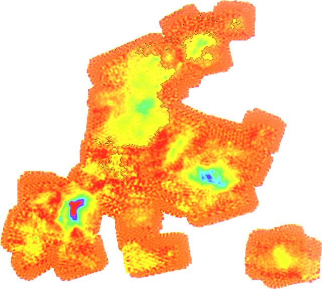 |
Figure 1. Map of 1.3 mm dust continuum emission covering about 2 pc in the ρ Ophiuchi cloud, with a resolution of 15″ (Motte et al 1998). The emission is proportional to column density, and the lowest contour corresponds to N ∼ 1.4 × 1022 cm−2 or Av ∼ 14 mag. Contour levels increase in spacing at higher levels (see Motte et al 1998 for details). The highest contour implies Av ∼ 780 mag. |
 |
Figure 2. The 850 µm emission and 450 µm to 850 µm spectral index distribution, covering about 7 pc with a resolution of 14″ at the northern end of the Orion A (L1641) molecular cloud (Johnstone & Bally 1999). The Orion Nebula is located directly in front of the strong emission at the center of the image. (Left) The 850 µm image showing the observed flux from −0.1 to 2 Jy/beam with a linear transfer function. The highest flux level corresponds roughly to Av ∼ 320 mag if TK = 20 K. (Center) The 850 µm image showing the observed flux from 100 mJy/beam to 20 Jy/beam with a logarithmic transfer function. (Right) The 450 µm to 850 µm spectral index in the range 2 to 6 with a linear transfer function. |
Interferometric arrays, operating at millimeter wavelengths, have provided unprecedented angular resolution (now better than 1″) maps of both molecular line and continuum emission. They are particularly critical for separating the continuum emission from a disk and the envelope and for studying deeply embedded binaries (e.g. Looney et al 1997, Figure 3). Complementary information has been provided in the infrared, with near-infrared star-counting (Lada et al 1994, 1999), near-infrared and mid-infrared spectroscopy of rovibrational transitions (e.g. Mitchell et al 1990, Evans et al 1991, Carr et al 1995, van Dishoeck et al 1998), and far-infrared continuum and spectral line studies (e.g. Haas et al 1995). Early results from the Infrared Space Observatory can be found in Yun & Liseau (1998).
The analytical tools for molecular cloud studies have grown gradually in sophistication. Early studies assumed LTE excitation, an approximation that is still used in some studies of CO isotopomers, but it is clearly invalid for other species. Studies of excitation require solution of the statistical equilibrium equations (Goldsmith 1972). Goldreich & Kwan (1974) pointed out that photon trapping will increase the average Tex and provided a way of including its effects that was manageable with the limited computer resources of that time: the Large Velocity Gradient (LVG) approximation. Tied originally to their picture of collapsing clouds, this approximation allowed one to treat the radiative transport locally. Long after the overall collapse scenario had been discarded, the LVG method has remained in use, providing a quick way to include trapping, at least approximately. In parallel, more computationally intensive codes were developed for microturbulent clouds, in which photons emitted anywhere in the cloud could affect excitation anywhere else (e.g. Lucas 1974).
The microturbulent and LVG assumptions are the two extremes, and real clouds probably lie between. For modest optical depths, the conclusions of the two methods differ by factors of about 3, comparable to uncertainties caused by uncertain geometry (White 1977, Snell 1981). These methods are still useful in some situations, but they are gradually being supplanted by more flexible radiative transport codes, using either the Monte Carlo technique (Bernes 1979, Choi et al 1995, Park & Hong 1998, Juvela 1997) or Λ-iteration (Dickel & Auer 1994, Yates et al 1997, Wiesemeyer 1999). Some of these codes allow variations in the velocity, density, and temperature fields, non-spherical geometries, clumps, etc. Of course, increased flexibility means more free parameters and the need for more extensive observations to constrain them.
Similar developments have occurred in the area of dust continuum emission. Since stellar photons are primarily at wavelengths where dust is quite opaque, a radiative transport code is needed to compute dust temperatures as a function of distance from a stellar heat source (Egan et al 1988, Manske & Henning 1998). For clouds without embedded stars or protostars, only the interstellar radiation field heats the dust; TD can get very low (5–10 K) in centers of opaque clouds (Leung 1975). Embedded sources heat clouds internally; in clouds opaque to the stellar radiation, it is absorbed close to the source and reradiated at longer wavelengths. Once the energy is carried primarily by photons at wavelengths where the dust is less opaque, the temperature distribution relaxes to the optically thin limit (Doty & Leung 1994):
 |
(14) |
where L is the luminosity of the source and q = 2 / (β + 4), assuming κ(ν) ∝ νβ.