3. BASIC PRINCIPLES OF DEBRIS FORMATION AND EVOLUTION

By definition, the tidal disruption of a satellite causes stars that used to be orbiting the satellite (which is in turn orbiting the parent galaxy) to become unbound and follow their own orbits around the parent galaxy. Fig 2 shows that, following disruption, the stars spread out through configuration space (i.e. they phase-mix, roughly along the satellite's orbit) as the distribution of orbital properties in debris corresponds to a distribution in orbital time-periods (described in Sect. 3.1). The rate at which the debris disperses reflects the scales over which debris orbital properties are distributed — which are set by the nature of tidal disruption (described in Section 3.2). The combination of tidal disruption and phase-mixing leads to phase-space morphologies for the debris that are primarily influenced by the mass of the satellite, its orbital path (which is in turn influenced by the parent galaxy potential), and the time since the debris became unbound. The scales of these morphologies can be broadly described by analytic formulae (Sect. 3.3.1) and represented by simple generative models (Sect. 3.3.2).

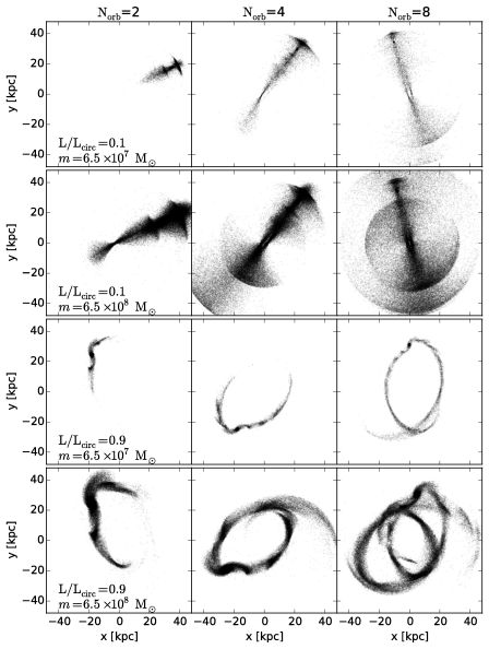Figure 2. Evolution of debris along highly (top panels) and mildly (bottom panels) eccentric orbits for two different mass satellites (labelled in left-hand panel). Note that highly eccentric orbits produce shells, while more circular orbits form streams.

3.1. Debris spreading: phase-mixing

The term phase-mixing beautifully encapsulates the physics of the evolution of debris structures. The nature of tidal disruption ensures that debris initially starts at the same phase (or position) along the orbit as the satellite from which it came, but with small offsets in its orbital properties (see Sect. 3.2). These offsets mean that the typical orbital frequency and time-periods in the debris differ systematically from those of the satellite, and hence that the debris will increasingly trail or lead the satellite in orbital phase as time goes by, mixing along the orbit to form streams and shells.

3.1.1. Intuition from spherical potentials

Figure 3 illustrates how and why phase mixing occurs for the idealized case of orbits in the spherical NFW profile potential used in our simulations. The top-left and upper-right-hand panels contour the radial time periods (time between successive apocenters or pericenters) and precession rate (angle between successive apocenters or pericenters) for orbits of a given energy and angular momentum per unit mass. The energy of a particle in a circular orbit, in a given (spherically symmetric) potential, is completely determined by the (constant) radius of that orbit. The orbital energy in Figure 3 is represented by the radius of the circular orbit with that energy. While the radial time periods depend much more strongly on energy than angular momentum, the precession angle depends more strongly on angular momentum, though to some extent on energy as well.

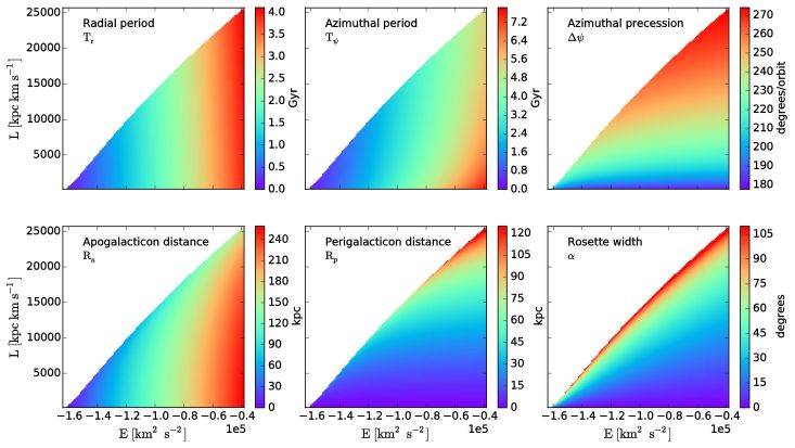Figure 3. Orbital properties in the spherical potential used in the N-body simulations as a function of energy (represented by the radius of a circular orbit of that energy) and angular momentum. The maximum angular momentum at a given energy is that of a circular orbit. The rosette width, α, is the angle the orbit travels through during half a radial period, centered around apocenter.

Figure 4 shows how a set of moderately eccentric orbits that have a small range of orbital energies (right panel) or angular momenta (left panel) diverge in phase over just a few orbits. In particular note that: orbits with the same angular momenta but different energies spread in radial phase (i.e. positions along their oscillation in radius between apocenter and pericenter), while those with the same energies but different angular momenta spread in precession angle; the physical spread is much more striking for energy differences than for the equivalent angular momentum differences because the precession rate is a much weaker function of orbital properties than the orbital frequencies; and there is little dependence on orbital phase of these observations.

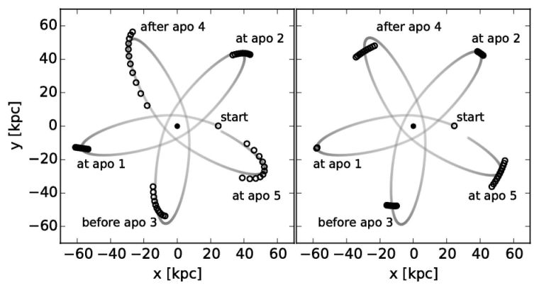Figure 4. Evolution of 11 particles that started at the same place along an orbit, but with a small spread in energy at fixed angular momentum (left hand panel) or angular momentum at fixed energy (right-hand panel). The orbit of a galactic satellite is shown by the solid line, and the galaxy's center is shown by the solid dot. The particles are shown at five subsequent times, one time for each petal of the orbit. Note that the positions of the particles diverge in phase in just a few orbits.

Figure 5 applies this intuition to one of our simulations, by color-coding particles with their differences in energy (first and third rows) and angular momentum (second and fourth rows) relative to the satellite from which they came. The sorting in energy along the orbital path and angular momentum around the orbital path is striking for both highly (top two panels) and mildly (lower two panels) eccentric orbits. It is also clear that the angular extent of the shells that form for the highly eccentric orbit is driven by differences in angular momenta, while the angular extent of streams is dominated by differences in energy.

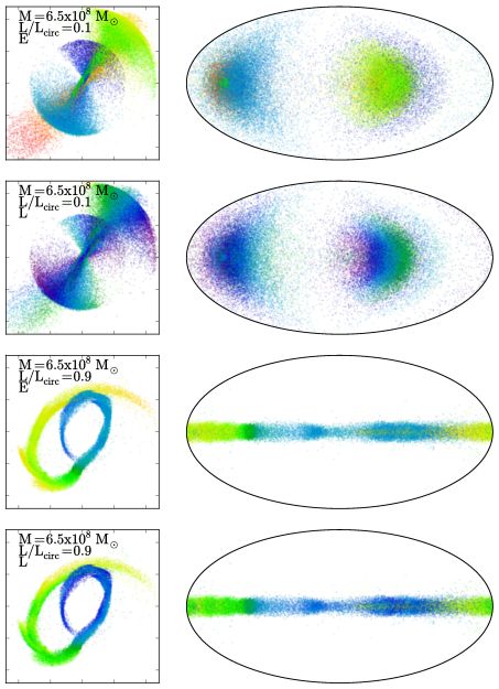Figure 5. Same as Fig. 1 but color-coded by differences between the satellite and debris in energy (first and third rows) and angular momenta (second and fourth rows).

3.1.2. Action-angle formalism

The description in the previous section is useful for developing an intuitive understanding of debris evolution since it employs familiar orbital descriptors (i.e., energy and angular momentum) that can be written down analytically for any potential and any point in phase-space. However, this description does not work for non-spherical potentials where angular momentum is not conserved and cannot be used to label orbits. Debris evolution can be described elegantly for more general (but integrable — see below) potentials using the action-angle variables of Hamiltonian dynamics. A formal development of this description is given in Helmi & White (1999) (and summarized in Binney & Tremaine (2008)). We restrict ourselves here to a summary of the key ideas and equations.

Any point in phase-space can be located using the traditional spatial and velocity co-ordinates (x, v). For regular (i.e. non-chaotic) orbits in integrable potentials, any phase space point can be equivalently labelled by conjugate variables (, ) where: (i) the actions, , are conserved orbital properties which fully specify the path of the orbit through phase-space; and (ii) the angles, , represent the position along the orbit at which the point lies. The actions and angles can be related through Hamilton's equations:

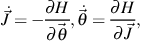(1)

where the function H (the Hamiltonian) is the energy of the orbit. Since the actions are conserved along an orbit ( = 0), ∂H / ∂ = 0 and hence the Hamiltonian H can only be a function of the actions, H = H(). Then the Hamiltonian defines three unique orbital frequencies associated with each angle,

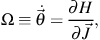(2)

which are also conserved along the orbit since they are only functions of . Equation (2) can be trivially integrated to give the position along the orbit at any time:

(3)

Note that these Hamiltonian angles are not trivially related to the angular position along an orbit derived from position (x, y, z): equation (3) shows that they increase linearly with time at a rate that is not orbital-phase dependent (i.e. with constant frequency), unlike, e.g., the angular coordinate along an eccentric orbit in a spherical potential, where the angular velocity is greater at pericenter than apocenter.

In this framework, the small range of orbital properties in tidal debris (illustrated with energy and angular momentum differences in Figure 3) can be represented by small changes to the actions, Δ , which in turn lead to a range in orbital frequencies,

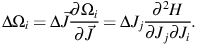(4)

This equation can also be trivially integrated to describe debris spreading (i.e. phase-mixing)

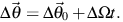(5)

This action-angle description allows a re-statement of our understanding of the origins of debris morphology in terms of the properties of the Hessian — ∂²H / ∂J_j∂J_i in equation (4) — which governs how orbital frequencies change in response to perturbations in the actions. This is a real symmetric matrix, which can be diagonalized and from which eigenvalues and eigenvectors can be derived. Assuming an isotropic distribution in actions (i.e. ΔJ the same in every dimension — not strictly true, see Sect. 3.2 and Bovy, 2014) the eigenvectors of the Hessian define the principal directions (in angle) into which debris spreading occurs and the eigenvalues define the rates at which this occurs. For realistic galactic potentials for which the Hessian has been derived, one eigenvalue has typically been found to dominate, indicating preferential spreading in just one dimension to form a tidal stream.

While action-angle variables offer an elegant description of debris dispersal, their versatility and applicability are not unlimited. Action-angles can be found for any spherical potential, but are only known for one family of non-spherical potentials: the triaxial Stäckel potentialsStäckel potentials (see Binney & Tremaine (2008)). Otherwise, they cannot generally be written down nor exactly derived numerically. This means that the transformation from (, ) to the more familiar co-ordinates (, ) is non-trivial and hampers the development of a simple intuitive understanding of how they correspond to each other. Moreover, this description breaks down entirely for chaotic regions of non-integrable potentials. Approaches to tackle these limitations typically involve approximating general potentials in which the actions are unknown with ones in which they are known. Examples include representing a general potential using an expansion in Stäckel potentials (Sanders 2012) or calculating actions for an orbit in a general potential from the actions derived for a set of orbits in a slightly perturbed potential (Bovy (2014), Sanders & Binney (2014)).

3.2. Orbital properties of tidal debris

The previous section attributed the dispersal of stars stripped from satellite disruption to the range in orbital time-periods within the debris. This section examines what sets that range.

Suppose a satellite of mass m_sat is following a circular orbit of radius R around a galaxy of mass M_R enclosed within R, with speed V_circ = √GM_R / R. Moving to a frame co-rotating with the orbit allows the definition of a time-independent effective potential, Φ_eff, and the conserved Jacobi integral, E_j = v² / 2 + Φ_eff. The tidal radius, r_tide, at which the size of the satellite is limited by the gravitational influence of the parent can be estimated from the saddle points (the inner and outer Lagrange points) in Φ_eff as:

(6)

(see Binney & Tremaine 2008, section 8.3 for derivation), which also defines a limiting E_j for escape from the satellite. However, since the escape of a star from the satellite depends on both its position and velocity, the tidal radius should not be considered as a solid boundary between bound and unbound stars. Moreover, it is not possible to define a strict tidal radius or E_j for satellites on non-circular orbits as there is no steadily-rotating frame in which the joint potential appears static. Nevertheless, numerical experiments have repeatedly demonstrated that the tidal scale,

(7)

suggested by equation (6) captures much of the physics that creates debris distributions from satellites of a variety of masses and on a variety of orbits (Johnston 1998, Helmi & White 1999, Eyre & Binney 2011, Küpper et al. 2012, Bovy 2014).

Figure 6 illustrates this understanding with plots of the orbital distributionsorbital distribution produced in our numerical simulations (see section 2), for satellites on orbits from highly eccentric to nearly circular (top panels, left to right). Each panel plots the energies (Δ E) and angular momenta (Δ L_z) of escaped particles (in blue) relative to the satellite's own (i.e. at origin in each plot — bound particles are shown in black). The axes have been scaled by simple estimates for the energy and angular momenta ranges over which the particles are expected to be distributed,

(8)

where Φ is the potential of the parent galaxy.

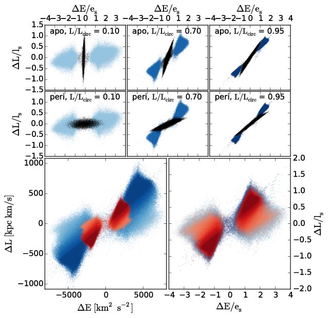Figure 6. Distribution in orbital properties for debris (blue) and satellite (black), relative to the satellite's orbit at apocenter (top row) and pericenter (second row). The illustrated orbits are for a 6.5 × 107 M⊙ satellite on orbits with L / Lcirc = 0.1, 0.7, 0.95. Left panels show the most eccentric orbits, and the most circular are on the right, with each case color-coded with a particular shade of blue. The axes in the top 2 rows are scaled by the expected energy and angular momentum scales given in equations (8). The blue points representing the debris are distributed similarly at apocenter and pericenter, for a given eccentricity. The bottom panels combine the energy and angular momentum distributions for all eccentricities and for two different masses (6.5 × 107 M⊙ in blue and 6.5 × 106 M⊙ in red) and plot them in physical units (bottom left) and scaled units (bottom right). Material that is still bound to the satellite is not shown in the lower two panels. Note that in scaled units (bottom right panel), the width of the leading/trailing distributions as well as the gap between them are similar across a wide range of eccentricities.

Each panel in Figure 6 shows paired distributions of unbound particles corresponding to debris leading/trailing the satellite along its orbit at negative/positive values of Δ E corresponding to systematically larger/smaller frequencies and shorter/longer orbital time periods. There is a distinct gap in orbital properties between the debris distributions for tidally stripped stars which is occupied by particles still bound to the satellite. (On the last pericentric passage, when all the particles become unbound the debris distribution will fill in this gap, see Johnston 1998). While the boundary between bound and unbound is not exact in configuration space, the separation between black and blue points in orbital properties is clear. The bottom panels contrast the debris distributions for all orbits (overplotted on each other) and two different satellite masses in physical (left-hand panel) and scaled (right-hand panel) units. All together, the figures show that both the width of the leading/trailing distributions and the gap between them are similar in these scaled units across a wide variety of eccentricities. Similar scaled distributions can be plotted for orbital actions and frequencies (see, e.g., Bovy 2014, for a discussion).

This uniformity in orbital properties for orbits with a range of eccentricities, when normalized with a single physical scaling, is one of the factors that enables the very simple descriptions of subsequent evolution outlined below in Sections 3.3.1 and 3.3.2. Since the satellite is typically small, the global potential is dominated by the (nearly static) parent galaxy and the debris orbital properties can be assumed not to evolve with time. Of course this assumption is a simplification — the gravitational influence of the satellite does not just turn off when a particle crosses the tidal radius but actually shapes the final distribution of debris orbital properties (see Choi et al. 2009, Gibbons et al. 2014, for some discussions of this).

3.3. Application: models of streams

3.3.1. Estimating physical scales in debris

The understanding of distributions of orbital properties in tidal debris (Sect. 3.2) can be combined with the behavior of orbits (i.e. the azimuthal time periods, T_Ψ, for increasing the azimuthal angle by 2π and precession angles between turning points, Ψ, see Fig. 3 and Sect. 3.1) to make simple predictions for the physical scales and time-evolution of the debris. Exploiting the fact that orbital time periods in spherical potentials are largely independent of angular momenta (as illustrated in Figure 3) the azimuthal time period for any orbit can be approximated by that of a circular orbit of the same energy T_Ψ^circ. Then, the angular extent of the debris at time t after disruption due to the characteristic energy scale over which it spreads (∼ 4 e_s — see equation [8] and Fig. 6) is of order:

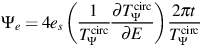(9)

Similarly, given the angle Ψ between subsequent apocenters along the orbit of the parent satellite, the angular extent due to the spread in apocentric precession rates over the characteristic angular momentum scale (∼ 4 l_s) can be estimated as:

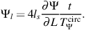(10)

Lastly, for a purely spherical potential, where the orbits are planar, the height h of debris perpendicular to the orbital plane is set by the range of orbital inclinations available to debris escaping at the Lagrange (i.e. saddle) points in the effective potential with the characteristic ranges in energies and angular momenta. It has been shown to be of the same order as the tidal radius,

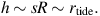(11)

These simple formulae can be used to characterize the length Ψ_e and width Ψ_l in and height h above the orbital plane for debris from a satellite of any mass disrupting along any orbit in any spherical potential (e.g. as confirmed with N-body simulations in Johnston et al. 2001). Note that, since both Ψ_e and Ψ_l are proportional to time, the ratio Ψ_e / Ψ_l is constant in time, and typically much greater than 1. This explains the tendency for debris to form streams (as also suggested by the unequal eigenvalues of the Hessian in the action-angle description). This ratio decreases for more eccentric orbits, which contributes towards the more shell-like appearance of debris in these cases (see section 4.1 for a more complete description).

3.3.2. Generating predictions for density distributions along streams

The understanding of orbits and orbital distributions in debris can also be combined to build more detailed predictions for the full phase-space distribution along tidal streams. One approach is to first integrate only the orbit of the satellite and subsequently calculate at each phase along the orbit the centroid, width and density of debris that material tidally stripped over time must have under some assumptions for the mass-loss history of the disrupting object. This was first done using approximate, analytic expressions for debris morphology, derived from energy and angular momenta considerations alone (as outlined above and in more detail in Johnston 1998, Johnston et al. 2001. Helmi & White 1999) instead followed how the density of a single packet of debris (i.e. unbound at the same point in time and at the same orbital phase) evolved using an action-angle formalism. More recently, Bovy (2014) and Sanders & Binney (2014) have built models in action-angle space, where the full phase-space distribution of a stream can be predicted by calculating the expected offset in angles at a given orbital phase from a single orbit integration. These latter models have the advantage over models built around energy and angular momenta in that they are also applicable to non spherical potentials and rely on a precise mapping rather than approximate scalings to calculate widths and offsets. However, they do rely on having methods to calculate actions and angles in arbitrary potentials, which introduce an additional layer of both complications and approximations (see Bovy 2014, Sanders & Binney 2014).

A second approach, slightly more computationally expensive but applicable to arbitrary potentials, is to integrate the satellite orbit and, at each time-step, release a set of particles to represent the stars lost at that time. At the point of release, the positions and velocites of the debris particles relative to the satellite are chosen to collectively reproduce the orbital distributions seen in full N-body simulations (e.g. as illustrated in Fig. 6). The particles' subsequent orbital paths in the combined field of the host and satellite can then be simply calculated using test-particle integration. At any point in time the integration can be stopped and the phase-space distribution of the particles be used to trace the resultant shells and streams. This simple approach has been used both for debris modeling (Yoon et al. 2011, Küpper et al. 2012) and potential recovery (Varghese et al. 2011, Gibbons et al. 2014).