


In this Appendix, we present all scattering calculations and results used in Section 5. Scattering in the atmosphere is a combination of Rayleigh scattering by molecules and Mie scattering by particulates. The scattering due to these two components can be dealt with individually. We begin by describing a general model for the scattering in a spherical atmosphere and then discuss the specific parameters needed to calculate Rayleigh and Mie scattering affecting observations from Las Campanas Observatory. Finally, we present the predicted contribution of scattered light to the program observations analyzed in this paper. We address zodiacal light and the integrated starlight as scattering sources separately.
The first calculations of radiative transfer in a Rayleigh scattering atmosphere were published by Chandresekar in 1950. Since then, a number of authors have published radiative transfer calculations addressing Rayleigh and Mie scattering in a curved atmosphere (e.g. Sekera 1952, Sekera & Ashburn 1953, and Ashburn 1954), and the effects of multiple-scattering (Dave 1964, de Bary & Bullrich 1964, and de Bary 1964). Careful measurements of zodiacal light over the sky and intensity distributions of the daytime sky have empirically demonstrated the accuracy of those calculations (e.g. Elterman 1966; Green, Deepak, & Lipofsky 1971; Weinberg 1964, Dumont 1965).
To calculate the atmospheric scattering affecting the observations
described in this Paper, we begin by adopting the scattering geometry
and coordinate system definitions used by Wolstencroft & van Breda
(1967, hereafter WvB67),
illustrated in Figure A1:
(A,
 )O
and (A',
)O
and (A',
 )X are
azimuth/zenith-distance
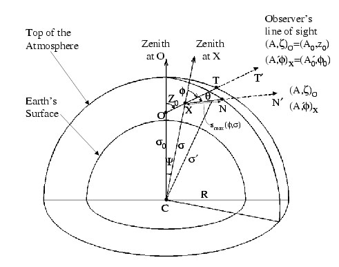
coordinate systems centered on the observer at O and a generic
point, X, along the line of sight, respectively. The problem is
then to calculate the brightness observed at O, along the line of
sight (A,
)O
= (A0, z0)O.
)X are
azimuth/zenith-distance
coordinate systems centered on the observer at O and a generic
point, X, along the line of sight, respectively. The problem is
then to calculate the brightness observed at O, along the line of
sight (A,
)O
= (A0, z0)O.
|
Figure A1. Geometry for atmospheric scattering along the line of sight OXT, with the observer at O and the line of sight exiting the atmosphere at T. In the case illustrated, scattering occurs at X from light entering the atmosphere at N from N'. |
Following WvB67, scattering occurs at the point X for radiation
which entered the atmosphere at the point N from the direction
N', given by (A,
)O
or (A',
)X. The light
arriving at X from N' can be expressed as

| (A1) |
in which the above-the-atmosphere source has flux
L(A', ), light
is attenuated by
e-Cext( ) h1(,
 ) as it
travels along NX, and s is the distance
along that path. Attenuation is a function of
Cext(),
the extinction cross section of the scattering particles in cm2,
and of h1(,
), the effective column
density of particles
along the line of sight. The effective column density is defined by
the local zenith angle, ,
and the distance, ,
which defines the point X relative to the center of the Earth
(see Figure A1):
) as it
travels along NX, and s is the distance
along that path. Attenuation is a function of
Cext(),
the extinction cross section of the scattering particles in cm2,
and of h1(,
), the effective column
density of particles
along the line of sight. The effective column density is defined by
the local zenith angle, ,
and the distance, ,
which defines the point X relative to the center of the Earth
(see Figure A1):
| (A2) |
in which
smax(,
) is the distance from
X to the top of the atmosphere at N, and
n(') is the
atmospheric number density of molecules in cm-3 as a function of
distance from the center of the Earth,
', and
as a function of the distance s' along the line XN.
The light scattered towards the observer from X is then
| (A3) |
in which
P( ) is the
scattering phase function and IX,
the flux arriving at point X is given in Equation
A1. Finally, the scattered light is further attenuated by the
factor
e-Cext()h2(z0,), in which
) is the
scattering phase function and IX,
the flux arriving at point X is given in Equation
A1. Finally, the scattered light is further attenuated by the
factor
e-Cext()h2(z0,), in which

| (A4) |
The total flux scattered into the line of sight (z0, A0) from sources distributed over entire visible hemisphere of the sky is then
| (A5) |
The visible sky at the point X dips below the observer's horizon at
large values of s. Hence, the limit of the integral over
, is
greater than /2 by the value
f () =
cos-1(R /
)
 14°, where R is
the radius of the Earth (6371 km). The
equations needed to change variables between
(A',) and
(z0, A0) are given WvB67.
14°, where R is
the radius of the Earth (6371 km). The
equations needed to change variables between
(A',) and
(z0, A0) are given WvB67.
The phase function for Rayleigh scattering is
P() = 1 +
cos2(). The
atmospheric density is given by the standard barometric formula
n() =
n0e-H/H0, where H
is the altitude above sea level (H =
- R), the scale
height is H0 = 7.99km, the density at sea level is
n0 = 2.67 × 10¹⁹
cm-3 , and the effective scattering cross-section for air is
Cscat = 7.78 ×
10-27( /
4600Å)-4cm2 (see
Schubert & Walterscheid
1999
and van de Hulst 1952).
For molecules in the atmosphere, extinction is entirely due to scattering,
so that Cext = Cscat. Atmospheric
extinction due to Rayleigh scattering is then
 R()
= Cext()
R()
= Cext()
 R
R n()
d. For the duPont
telescope at Las Campanas, which is at an altitude of 2.28 km, the
expected Rayleigh extinction is
R(4600Å) = 0.12.
n()
d. For the duPont
telescope at Las Campanas, which is at an altitude of 2.28 km, the
expected Rayleigh extinction is
R(4600Å) = 0.12.
The phase function for Mie scattering by particulates in the
atmosphere depends on the distribution of particle sizes, and must be
empirically determined. We adopt the phase function measured by
Green, Deepak & Lipofsky
(1971)
from their complete analysis of the
Mie (particulate) scattering and Rayleigh (molecular) scattering
components of the atmosphere based on the scattering of sunlight.
Their results are in good agreement with theoretical scattering models
and other estimates of the size-distribution of particles in the
atmosphere and have a negligible dependence on wavelength for our
purposes (see
Elterman 1966, and
Deepak & Green 1970).
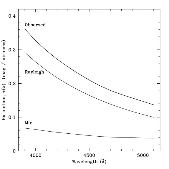
The scattering and extinction coefficients for particulate scattering are
a function of the size distribution of particles and vary with time
and geography. The extinction due to Mie scattering can, however, be
inferred from the observed extinction for a point source and the
calculated Rayleigh extinction coefficient:
M =
obs -
R ~ 0.05 at
4500Å (see Figure A2). This value is in
good agreement with estimates for
Tenerife by Dumont (1965)
and for
Haleakala by Weinberg (1964).
This is not surprising as our observed
obs() is consistent with the
CTIO curves
(Baldwin & Stone 1984,
Stone & Baldwin 1983),
and
R() is simply a
function of the atmospheric density.
|
Figure A2. We compare the observed
extinction,
|
Unlike the case for molecules, the attenuation caused by particulates
is not entirely due to scattering.
Staude (1975)
adopts values of Cscat = 4.47 × 10⁻¹¹
cm2 and Cext = 7.53 × 10⁻¹¹
cm2 for dry air at 4200Å. With a sea level density of
n0 = 1.11 × 104cm3, and a
distribution scale
height of only h0 = 1.2 km, these parameters give
M ~ 0.01 at 2
km. We have scaled Cscat and
Cext to give values consistent with our observed value of
M. Scaling
H0 or assuming a different value of
H would have the same effect on
IMscat(, ZL).
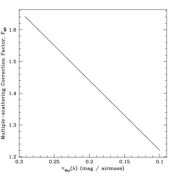
The scattering model discussed above describes a single scattering event.
However, multiple scattering events become significant for scattering
angles
 30°
(de Bary 1964,
de Bary & Bullrich 1964).
Consequently, we apply a multiple scattering correction for
Rayleigh scattering which is adopted from
Dave (1964)
and plotted in
Figure A3. The correction factor
plotted in Figure A3 is simply the factor by
which the intensity of
scattered light increases over the single-scattering case. Multiple
scattering does not occur due to particulates (Mie case) because
of the small scattering angles which dominate that process and
very small values of
M().
30°
(de Bary 1964,
de Bary & Bullrich 1964).
Consequently, we apply a multiple scattering correction for
Rayleigh scattering which is adopted from
Dave (1964)
and plotted in
Figure A3. The correction factor
plotted in Figure A3 is simply the factor by
which the intensity of
scattered light increases over the single-scattering case. Multiple
scattering does not occur due to particulates (Mie case) because
of the small scattering angles which dominate that process and
very small values of
M().
|
Figure A3. Correction factor for multiple scattering, FMS, as a function of the Rayleigh extinction. |
To confirm the accuracy of our calculations, we checked our scattering
model against published results of
Staude (1975),
WvB67, and
Ashburn (1954)
for a uniform, sky-filling source of unit flux. We find that our
results are consistent to within 4% for zenith angles
z 80°
before the multiple scattering correction is applied. (WvB67 predates
evidence for the effects of multiple scattering, and Staude adopts the
same corrections used here.) The uncertainty in the multiple
scattering correction is roughly 4-7%, increasing with larger values
of .
Using the expressions above, we calculate the scattered light flux,
Iscat(), resulting from Mie scattering by particulates
and Rayleigh scattering by molecules throughout the nights of our
observations. The results depend explicitly on the absolute position
of the Sun and the Galactic center relative to the observatory and
relative to the target field. In the following sections, we consider
the cases of zodiacal light (ZL) and integrated starlight (ISL) as the
extra-terrestrial source of flux separately.
To calculate the scattered zodiacal light along the line of sight of
our observations, we adopt values for the zodiacal flux given in
Leinert et al. (1998),
which are taken from
Levasseur-Regourd & Dumont
(1980)
with values at elongations
 < 30° added
from space-based observations. These ZL values are above-the-atmosphere
fluxes and are in excellent agreement with later space-based results
(see Leinert et al.
1981).
To obtain a smooth flux distribution of ZL
on the sky (see Figure A4), we use the spherical
interpolation method developed by
Renka (1997).
< 30° added
from space-based observations. These ZL values are above-the-atmosphere
fluxes and are in excellent agreement with later space-based results
(see Leinert et al.
1981).
To obtain a smooth flux distribution of ZL
on the sky (see Figure A4), we use the spherical
interpolation method developed by
Renka (1997).
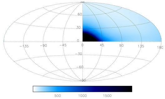
|
Figure A4. Zodiacal light over the sky is
plotted in sun-centered ecliptic coordinates, so that the Sun is at
( |
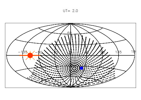
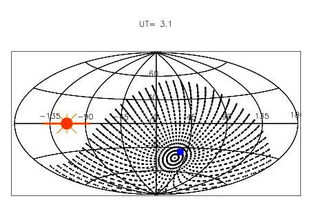
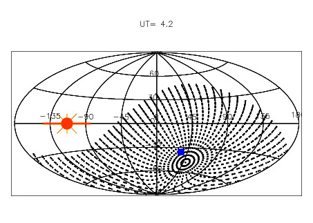
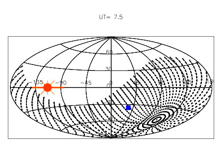
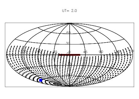
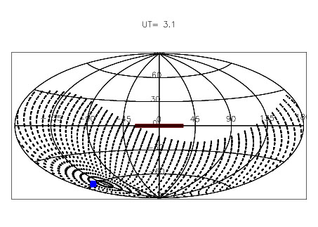
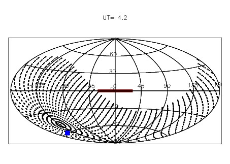
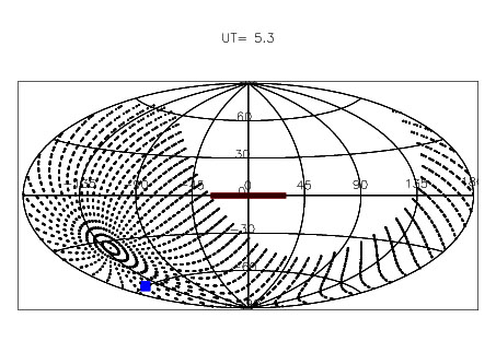
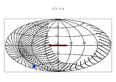
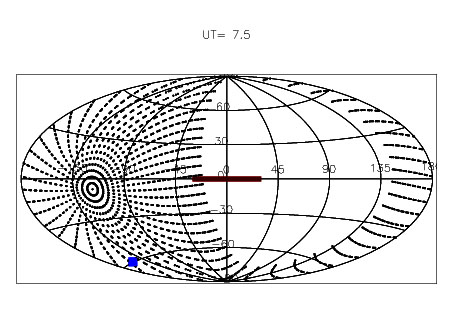
In Figure A5, we show the integration pattern
in (zenith angle) and
A' (azimuth) used to calculate
Iscat(,
ZL) (Equation A6) at the indicated
times during the nights of our observations. Actual calculations were
done with twice the number of integration points shown in the figures.
The visible part of the sky (shown by the integration pattern) is
at least 30 degrees from the Sun during our observations.
| 
| 
|

| 
| 
|
Figure A5. Integration pattern for calculating scattered zodiacal light. Each plot is an Aitoff projection of the sky in Ecliptic coordinates. The position of the Sun and the ecliptic plane are indicated by the Sun symbol with a bar through it. Obviously, the ecliptic plane is along the 0° latitude line. Our target field is indicated by the square. The ecliptic coordinates of the zenith can be seen as the "bullseye" center of the integration pattern. The motion of the target relative to the local zenith is clear as the target moves from east to west of the zenith point in the integration pattern. The coordinates of the local horizon are traced by the edge of the integration pattern. The Sun is obviously located just to the west of the horizon at the start of the night (UT = 2.0 hr) and just to the east of the horizon at the end of the observing night (UT = 7.5 hr). | ||
As a technical detail, we have made the simplifying assumption that
the spectral shape of the ZL over the visible hemisphere is
uniform. That is, only the mean flux of the ZL changes. Although
there are variations in the color (defined in Equation 1)
of the ZL over the range 3900-5100Å from
= 30° to
= 180°, the
total change is empirically less than ~ 8% and our target is in the
center of the expected color range (e.g.,
Frey et al. 1974,
Leinert et al. 1981).
We have run trail scattering models in which we change the flux with
over the
sky by ± 4%, and we find that the effect on the predicted
scattered flux is changed by 0.4% at airmasses higher than 1.6, and
0.2% at the lowest airmass. In other words, by ignoring the color
variation in ZL over the sky, the scattered light model will be wrong
by 0.2% at 3900Å relative to the value at 5100Å, or ± 0.1%
over the range 3900-5100Å for our observing situation
(positions of the Sun relative to the target and the horizon).
|
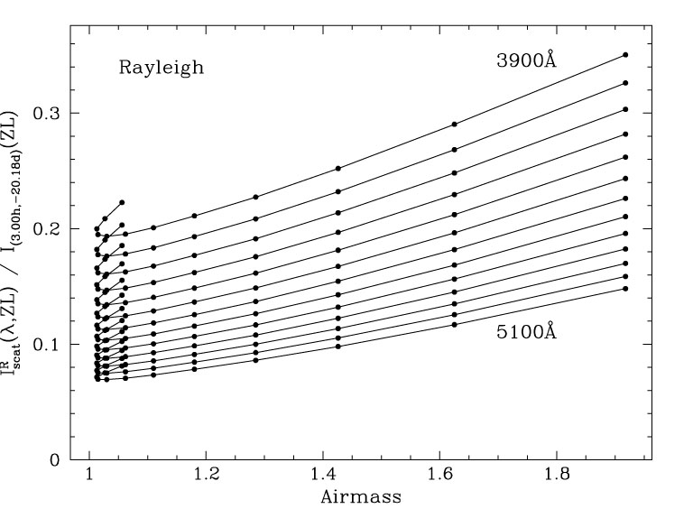
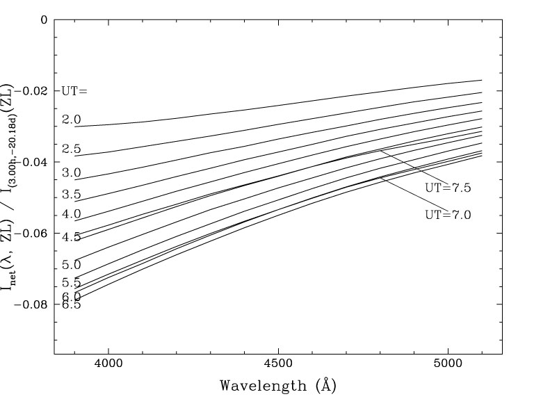
Figure A6. The Rayleigh scattered zodiacal
light contribution to our observed night sky flux
on the nights of 1995 November 27-29 as a function of airmass at
100Å intervals from
3900Å to 5100Å. Flux decreases monatonically with wavelength
at any airmass, following the behavior of
( |
|
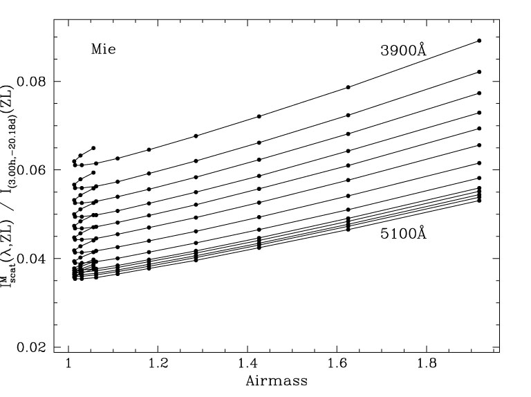
Figure A7. Same as Figure A6, but here we plot the contribution of Mie scattered zodiacal light along the line of sight. Again, the scattered light flux is plotted as a fraction of the above-the-atmosphere zodiacal light flux in our target field. |
|
Figure A8. Same as
Figure A6, but
here each line indicates
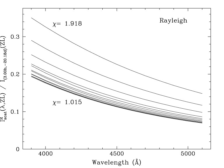
IRscat( |
|
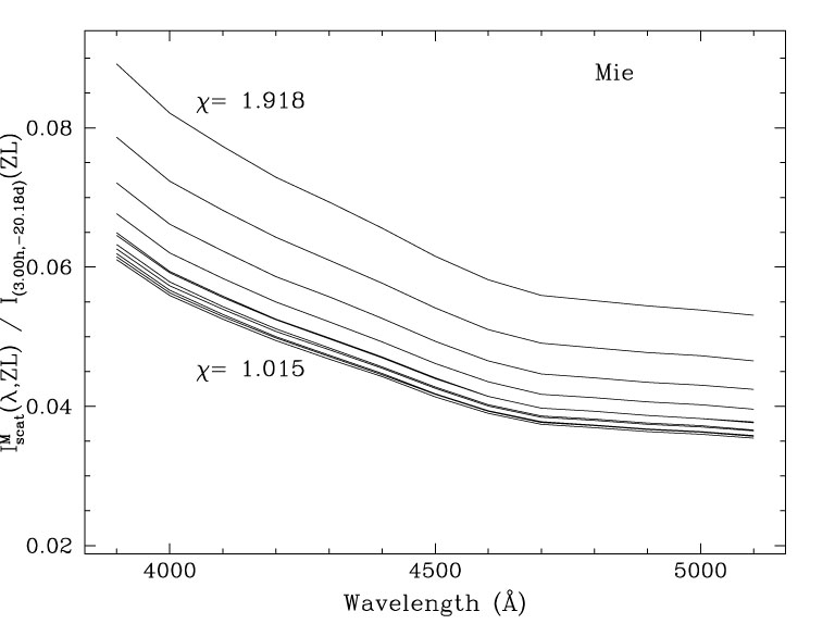
Figure A9. Same as Figure A8, but showing the Mie scattered zodiacal light. |
The predicted Rayleigh and Mie scattering flux of ZL,
IRscat and
IMscat, respectively, along the line of
sight to our target field throughout our observations is shown in
Figures A6 -
A9. In
those Figures, we show the scattered light as a function of the
above-the-atmosphere ZL flux in target field at
( = 3.00 h,
 = - 20.18 d),
I(3h, - 20d)(ZL).
This removes the spectrum of the ZL
and highlights the wavelength dependence of Iscat.
The predicted scattered flux is not symmetric about the zenith because
the distribution of ZL over the sky is not symmetric: the scattered
light will be smaller at the same airmass if the Sun is further below
the horizon, i.e. the middle of the night. The scattered flux is
therefore minimized near UT ~ 4, when the field is still at low
airmass and the brightest regions of the ZL are below the horizon. In
Figure A10, we show the total combined effect
of the atmosphere on the ZL flux received from the target field:
= - 20.18 d),
I(3h, - 20d)(ZL).
This removes the spectrum of the ZL
and highlights the wavelength dependence of Iscat.
The predicted scattered flux is not symmetric about the zenith because
the distribution of ZL over the sky is not symmetric: the scattered
light will be smaller at the same airmass if the Sun is further below
the horizon, i.e. the middle of the night. The scattered flux is
therefore minimized near UT ~ 4, when the field is still at low
airmass and the brightest regions of the ZL are below the horizon. In
Figure A10, we show the total combined effect
of the atmosphere on the ZL flux received from the target field:
| (A6) |
|
Figure A10. The net effect of the
atmosphere on the observed spectrum of zodiacal light.
Inet(ZL) is the flux
received from the target field plus the scattered light coming from
the entire visible hemisphere of the sky:
Inet( |
Finally, from
Inet(,
ZL) we can calculate an effective
extinction for the ZL from our target field at the specific times at
which our observations occurred. The effective extinction is defined
by the equation

| (A7) |
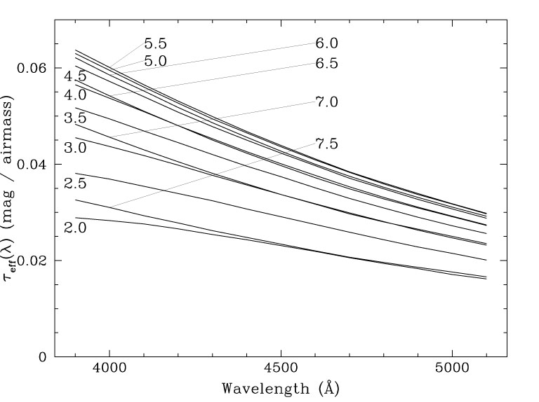
The effective extinction is plotted in Figure A11, and is specific to our target field, times of observation, observed extinction, geographic latitude and longitude, and altitude.
|
Figure A11. Each line shows the effective extinction for the zodiacal light as a function of wavelength for our observations at the indicated UT. The effective extinction corresponds to the net loss of light relative to the above-the-atmosphere flux of the zodiacal light in our field of view (see Figure A10). For comparison with the total observed extinction derived from standard stars see Figure 4. |
The result which is applied to our ZL measurement from the modeling
discussed here is
eff(, t), which
corresponds to
Inet(,
t, , ZL) rather
than
Iscat(,
t,, ZL). The
virtue of this approach is that
the absolute flux accuracy of the adopted ZL over the sky
(Fig. A4) does not affect our results; only the
accuracy of the relative flux distribution over the sky matters.
In the regions of the sky which dominate the scattering for our
observations (solar elongations of
> 30°), the
relative
flux errors for the ZL over the visible hemisphere of the sky are
5% over large areas (>
30°), and better on small scales.
Such errors will propagate into final measurement of the ZL at the
level of < 1% at high airmass, and < 0.4% at low
airmass. Nevertheless, we note that the above-the-atmosphere value of
the ZL from
Levasseur-Regourd & Dumont
(1980)
agrees with our measurement in our target field to within 2%.
, ZL) rather
than
Iscat(,
t,, ZL). The
virtue of this approach is that
the absolute flux accuracy of the adopted ZL over the sky
(Fig. A4) does not affect our results; only the
accuracy of the relative flux distribution over the sky matters.
In the regions of the sky which dominate the scattering for our
observations (solar elongations of
> 30°), the
relative
flux errors for the ZL over the visible hemisphere of the sky are
5% over large areas (>
30°), and better on small scales.
Such errors will propagate into final measurement of the ZL at the
level of < 1% at high airmass, and < 0.4% at low
airmass. Nevertheless, we note that the above-the-atmosphere value of
the ZL from
Levasseur-Regourd & Dumont
(1980)
agrees with our measurement in our target field to within 2%.
To evaluate the accuracy of our calculated values of
Inet(ZL) (see Equation A7), we estimate that the
uncertainty in our scattering calculations is 8% at the low zenith
angles (< 30°) where the bulk of our observations occur. This
estimate is based on the comparisons between scattering models and
atmospheric measurements presented in
Green et al. (1971),
Dave (1964),
and Staude (1975),
and is consistent with the uncertainties discussed
in WvB67,
Ashburn (1954), and
Sekera & Ashburn (1953).
The time-weighted average of Iscat(ZL) over the
course of our observations is ~ 0.15 × I(3h, -
20d)(,
ZL), so Iscat(ZL) has an uncertainty of
1.2% of the ZL flux in our target field.
The uncertainty in the observed extinction is much less than 1% and
adds negligibly to this error. See Section 6 for
further discussion of the accuracies of the zodiacal light measurement.
We can also assess the accuracy of
eff()
independently from our own data, as discussed in
Section 5. Notice that
Inet(ZL) changes with time in a way which is
only weakly
dependent on wavelength. A consistent solution for the ZL with both
wavelength and airmass will be strong confirmation of the accuracy of
the values for
eff(, t) calculated here.
Unlike the scattered ZL, the scattering which results from integrated starlight (ISL) must be incorporated into our analysis of the observed night sky spectrum as an absolute flux value. We must therefore first derive a spectrum for the ISL as a function of position over the sky. To do so, we have followed the method suggested by Mattila (1980a, 1980b), which we briefly summarize here.
The spatial and flux distribution of stars of all spectral types can be described by exponential distributions perpendicular to the Galactic plane (in the z direction) and narrow Gaussian distributions in intrinsic magnitude. The mean emission per pc3 from stars of type i as a function of distance from the Galactic plane, z, can be written as

| (A8) |
in which Di(0) is the number density of stars per
cubic parsec in
the plane, hi is the scale height of the vertical
distribution,
and Mi is the mean absolute magnitude of the spectral
type i. The observed flux is also attenuated by interstellar
extinction, which can be expressed by a two-component extinction law
characterized by a total extinction
a0()
= a1()
+ a2(),
with
a1():
a2()
in the ratio 1.84 : 0.62
(Neckel 1965).
The z-dependence of extinction can be written as

| (A9) |
for z given in parsecs
(Neckel 1965,
Neckel 1980).
We find a good
fit to the observed ISL by adopting standard values for
a0()
(Zombeck 1990),
scaled to a0(V) = 1.5 mag kpc-1.
In cylindrical coordinates, the flux per unit solid angle (ergs s-1 cm-2 sr-1 Å-1) from stars fainter than m0 along the line of sight at Galactic latitude b can be expressed by the volume integral
| (A10) |
in which r is the distance along the line of sight from the observer
in parsecs and fi is the spectral energy density of a
star of type
i in ergs s-1 cm-2 Å-1. In
the derivation of the above integral, the
1/4 r2 loss
of flux from each star along the line of sight has canceled
with the r2
d
r2 loss
of flux from each star along the line of sight has canceled
with the r2
d in the
volume integral, and we have changed
variables using the relation
r = z/sinb. The lower limit of
integration is simply the distance modulus for stars of each type
corresponding to the bright magnitude cut-off, m0, so
that z0 = 100.2(m0 - Mi +
5) in parsecs. Finally, the extinction from z to the
observer is
in the
volume integral, and we have changed
variables using the relation
r = z/sinb. The lower limit of
integration is simply the distance modulus for stars of each type
corresponding to the bright magnitude cut-off, m0, so
that z0 = 100.2(m0 - Mi +
5) in parsecs. Finally, the extinction from z to the
observer is
| (A11) |
Using 33 individual stellar types described by the parameters
Mi, Di, and hi from
Wainscoat et al.
(1992),
we obtain integrated
spectra which agree with the observed star counts at V and B
(Roach & Megill 1961,
see also
Allen 1973)
to m0 = 6 V mag at
|b| > 5° to better than 10%, which is more than adequate
for our purposes. The spectral energy densities for each stellar type,
fi()
were obtained from the STScI archive
(Jacoby, Hunter, &
Christian 1984)
and have a resolution of roughly 4Å. We include
stars by type with m0 < 6 V mag from the SAO
star catalog
by hand. We felt this was necessary as the statistical variation in
stellar density on small scales around the solar neighborhood can have
a significant impact on the accuracy of the model, while variations
are apparently averaged out in stellar populations at large distances.
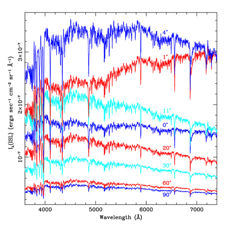
In Figure A12, we plot the total integrated
starlight (ISL) with no bright magnitude cut off at
0° < |b| < 90°. The total flux at
|b| = 90° is roughly 20 × 10-9 ergs
s-1 cm-2 sr-1 Å-1,
while the flux near the plane is as high as 300 × 10-9
ergs s-1 cm-2 sr-1
Å-1.
Interstellar extinction limits the ISL flux in the plane in our
model, probably more than is appropriate. However the flux rises
rapidly even 1° degree above the plane to more realistic
values. The limited sky area at b = 0° precludes this from
impacting the accuracy of the models.
|
Figure A12. The mean integrated starlight (ISL) spectra as a function of Galactic latitude (as labeled) produced by the model described Section A.3. |

|
Figure A13. Integrated starlight over the sky from star counts at V. Flux units are 1 × 10⁻⁹ ergs s-1 cm-2 sr-1 Å-1. |
| 
| 
|
| 
| 
|
Figure A14. Integration pattern for the calculation of scattered ISL flux. Each plot is an Aitoff projection of the sky in Galactic coordinates. The center of the Galaxy is at the center of each plot (l = 0°, b = 0°). The Galactic plane within 30 degrees of the Galactic center is marked by the thick line. Our target field is indicated by the square. The Galactic coordinates of the zenith can be seen as the "bullseye" center of the integration pattern. The coordinates of the local horizon are shown by the edge of the integration pattern. The Galactic plane is running along the horizon at the start of the night (UT = 2.0 hr), and is perpendicular to the horizon at the end of the night (UT = 7.5 hr). The Galactic center is never above the horizon. See Figure A5 for further discussion. | ||
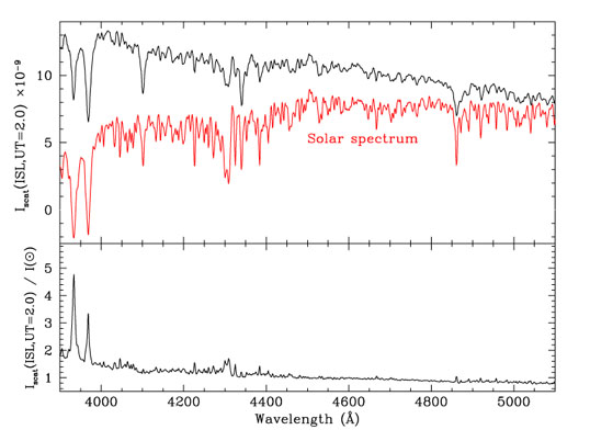
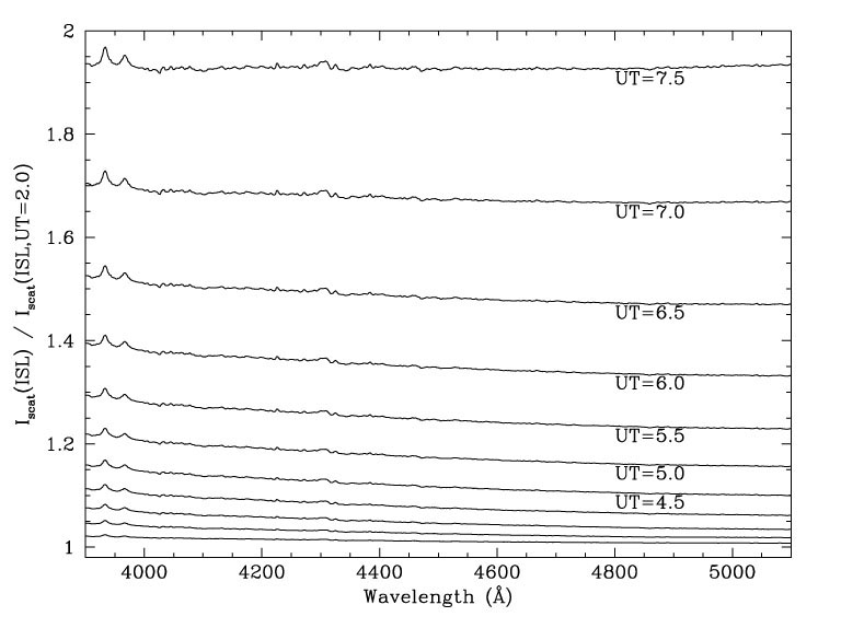
Figure A15 shows the total scattered ISL flux
due to
Rayleigh and Mie scattering which contributes to observations of our
target field at the beginning of the observing night (UT = 2.0 hr). The
total flux (~ 12 × 10-9 ergs s-1
cm-2 sr-1 Å-1) is roughly 12% of
the ZL flux above the atmosphere in our target field. The ISL flux in the
observed sky spectrum will impact our measurement of the ZL flux only
if the ISL spectrum has the same features as the solar (zodiacal
light) spectrum. In the lower plot of
Figure A15,
we therefore plot ratio of the
Iscat(,
t, , ISL) to
the solar spectrum, normalized at 4600Å. It is clear from
this plot that the scattered ISL and solar spectra differ by 5-10%
at > 4500Å, but by a factor of 3-5 in the strength of spectral
features
at less than 4500Å. In Figure A16, we
plot the ratio of
Iscat(,
t, , ISL)
throughout the night to
Iscat(,
t, , ISL) at UT
= 2.0 hr. From this
plot it is clear that strength of spectral features changes only very
weakly throughout the night, by < 1% over the majority of the spectrum
and by < 4% at 3900-4000Å (CaI H & K). The consistency of our ZL
measurement (Section 6) over the full wavelength
range 3900-5100Å is, therefore, a strong test of the accuracy of the
predicted contribution of scattered ISL. As discussed in
Section 5, the predicted scattered ISL flux is
entirely
consistent with our observations. See Section 5
for further discussion.
|
Figure A15. The upper plot shows the predicted spectrum of the scattered ISL along the line of sight to the EBL field at UT = 2.0 hr for our observations. Units are ergs s-1 cm-2 sr-1 Å-1. The solar spectrum is also shown, scaled to the same flux and offset, to allow visual comparison of the spectral features. The lower plot shows the ratio of that spectrum to the solar spectrum, normalized at 4600Å, the center of our observed wavelength range. Note that the total flux from the scattered ISL in this case is < 5% of the total flux of the combined zodiacal light and airglow, and the spectral features are weaker in the scattered ISL. |
|
Figure A16. The ratio of the predicted scattered ISL spectrum at the indicated UT on the night of our observations, relative to the predicted spectrum at UT=2.0 hr. The plot demonstrates that relatively small changes (< 4%) occur in the strength of individual spectral features over the night, while changes in broad-band color and mean flux are significant. |
Obviously, the model we describe above makes no allowance for variation in the ISL with Galactic longitude. For comparison, we show in Figure A13 an Aitoff projection of the ISL from star counts over the sky, which shows that the ISL has only minor dependence on longitude at b > 20°. At lower latitudes where the variation is greater with longitude, the spectroscopic model we employ does give a good approximation to the average ISL. Because the contribution to the scattering comes from a wide spread in longitude (compare Figures A14 and A13), the mean value is adequate for our purposes. To test this, we ran simulations in which we maintained the mean ISL flux with latitude, but varied the ISL flux with longitude by ± 25%. We find that the total scattered ISL is affected by less than 9% throughout the night due to longitudinal variations around the mean.
The mean flux in our models for the ISL is consistent with the star
counts of
Roach & Megill (1961)
to within ± 10% at both V and
B. As in the previous section, we estimate that the
uncertainty in our scattering calculations is 8% at the low zenith
angles (< 30°) where the bulk of our observations occur.
Combining these, we estimate the uncertainty in
Iscat(,
t,, ISL) to be
13%. As the relative mean
strength of spectral features in starlight is 0.6-4% of the total ZL
flux in our target field at the 4000 - 5200Å, this corresponds to an
uncertainty of < 0.5%.
Any significant errors in our model, either in mean flux as might be caused by longitudinal variations in the ISL, or in the spectral energy distribution, would show up as inconsistencies in the solution for the ZL flux as a function of wavelength. Furthermore, errors would be worst at higher airmass, where Figure A14 shows that the low-galactic-latitude sky has a greater impact on the scattered ISL, the mean flux is greater, and the stellar-type mix is more sensitive. No such variations with wavelength are found, as we have discussed in Section 5. See Section 6 for further discussion of the accuracies of the zodiacal light measurement.
 = 0°,
= 0°,
 = 0°),
the anti-solar direction is
(
= 0°),
the anti-solar direction is
(