


The bootstrap was invented by Efron in 1977 (e.g., see Efron 1979). The method uses the enhanced computing power available in this age to explore statistical properties that are beyond the reach of mathematical analysis. At the heart of this method is the procedure of creating from the available data set, hundreds or thousands of other "pseudo-data" sets. In older methods one assumed or derived some parametric distribution for the data and derived statistical measures. With bootstrap, any property of the original data set can be calculated for all the pseudo-data sets and the resulting variance of a measured quantity calculated over the entire ensemble. We have applied the bootstrap resampling technique (to my knowledge for the first time in astronomy) to illustrate its use in estimating the uncertainties involved in determining the galaxy-galaxy correlation function (Barrow, Bhavsar and Sonoda 1984).
The two-point correlation for galaxies is the factor by which the number of observed galaxy-galaxy pairs exceed the number expected in a homogeneous random distribution, as a function of their separation. It is an average taken over the entire sample and measures the clumping of galaxies in the universe. Usually a galaxy's coordinates in the sky are relatively easy to measure and known accurately. The same cannot be said for a galaxy's distance from us which is a difficult and time consuming measurement. Thus the most common catalogs available are sky surveys, for which the two-point correlation function has been extensively determined; though in the last few years 3-D spatial catalogs of limited extent have become available.
With a sky catalog one measures the angular two-point correlation function. This was pioneered by Totsuji and Kihara (1969), and Peebles (1973) and followed up extensively by the work of Peebles (1980) and his collaborators. They found that the angular correlation function for galaxies is a power law. If the projected distribution has a power law correlation then the spatial two-point correlation is also a power law with a slope that is steeper by -1 than the angular correlation (Limber 1953). The angular two-point correlation for galaxies to magnitude limit 14.0 in the Zwicky catalog (Zwicky et al. 1961-68) is given by
| (1) |
Let me describe in a little more detail the actual determination of
the above measurement. The sky positions (galactic longitude and
latitude) of all galaxies brighter Than apparent magnitude 14.0 and in
the region
 > 0° and
b" > 40°
forms our sample. This consists of 1091
galaxies in a region of 1.83 steradian. The angular separation between
all pairs of observed galaxies is found and binned to give
Noo(
> 0° and
b" > 40°
forms our sample. This consists of 1091
galaxies in a region of 1.83 steradian. The angular separation between
all pairs of observed galaxies is found and binned to give
Noo( ), the
number of pairs observed to be separated by
. This is compared
to the expectation for the number of pairs that would be obtained if the
distribution was homogeneous, by generating a Poisson sample of 1090
galaxies in the region and determining the pair-wise separations
between each of the observed 1091 real galaxies and the 1090 Poisson
galaxies. This gives us
Nop(),
the number of pairs between observed and Poisson galaxies separated by
. The angular two-point
correlation function is
), the
number of pairs observed to be separated by
. This is compared
to the expectation for the number of pairs that would be obtained if the
distribution was homogeneous, by generating a Poisson sample of 1090
galaxies in the region and determining the pair-wise separations
between each of the observed 1091 real galaxies and the 1090 Poisson
galaxies. This gives us
Nop(),
the number of pairs between observed and Poisson galaxies separated by
. The angular two-point
correlation function is
| (2) |
The binning procedure is decided upon before performing the
analysis. The data is binned so that there are roughly an equal
number of observed-Poisson pairs in each bin. A plot of
log  () versus
log shows the
correlation function to be a power law. The
slope of the best fitting straight line determined by some well
defined statistical measure gives the value of the exponent in
equation (1). Our independent determination of this exponent gives a
value of 0.77, consistent with earlier determinations. The question
is: from the limited data available, how accurately does this describe
the correlation function for galaxies in the universe? It is assumed
that our sample is a "fair sample" of the universe
(Peebles 1980),
implying our faith in the assumption that the region of the universe
that we sample is not perverse in some way. The formal errors on the
power law fit to the data do not give us the true
variability in the
slope of the correlation function that may be expected. These formal
errors indicate to us a goodness of fit for the best power law that we
have found to fit the data; but the question of the statistical
accuracy of the value 0.77 representing the slope of the power law for
the two-point correlation function for galaxies in the universe,
remains uncertain.
() versus
log shows the
correlation function to be a power law. The
slope of the best fitting straight line determined by some well
defined statistical measure gives the value of the exponent in
equation (1). Our independent determination of this exponent gives a
value of 0.77, consistent with earlier determinations. The question
is: from the limited data available, how accurately does this describe
the correlation function for galaxies in the universe? It is assumed
that our sample is a "fair sample" of the universe
(Peebles 1980),
implying our faith in the assumption that the region of the universe
that we sample is not perverse in some way. The formal errors on the
power law fit to the data do not give us the true
variability in the
slope of the correlation function that may be expected. These formal
errors indicate to us a goodness of fit for the best power law that we
have found to fit the data; but the question of the statistical
accuracy of the value 0.77 representing the slope of the power law for
the two-point correlation function for galaxies in the universe,
remains uncertain.
The bootstrap method is a means of estimating the statistical accuracy of the two-point correlation from the single sample of data. A pseudo data set is generated as follows. Each of the 1091 galaxies in the original data is given a label from 1 to 1091. A random number generator picks an integer from 1 to 1091, and includes that galaxy in the pseudo data sample. A galaxy is picked from the original data in this manner through 1091 loops. The pseudo data sample will contain duplicates of some galaxies and will not contain all the galaxies of the original data set. The angular correlation function can be calculated for this new data set in exactly the same manner as the original by fitting it to a power law of the form

| (3) |
This entire procedure of generating a new data set and determining
its angular correlation can be repeated hundreds of times using
different sets of random numbers. The samples generated in this way
are called bootstrap samples. The frequency distribution for the
values of the slope,
 , and the
correlation length,
0,
can be plotted
for the ensemble of bootstrap samples to estimate the variance of
,
and 0
respectively.
, and the
correlation length,
0,
can be plotted
for the ensemble of bootstrap samples to estimate the variance of
,
and 0
respectively.
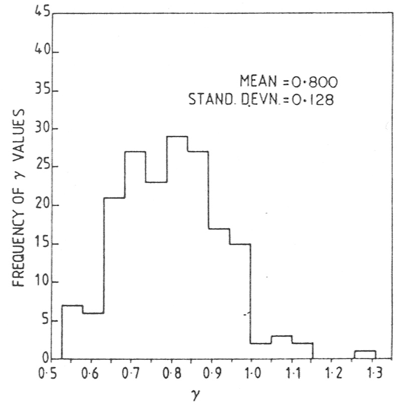
We generated 180 bootstrap samples for the 1091 galaxies in the
Zwicky data, determined the two-point correlation function for each as
described by equation (2), and fit the power law described by equation
(3) to each correlation function. Figure 1 shows
the distribution of
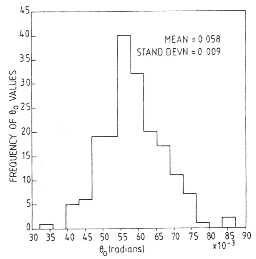
obtained for these 180 samples. Figure 2 shows
the distribution of
0.
|
| Figure 1. |
|
| Figure 2. |
We can determine the standard deviation in the values of
and
0. These are
found to be

| (4) |

| (5) |
This means that 68 percent of the values of
lie in an
interval
whose width is 0.26, or in other words, the bootstrap samples show that 68%
of the lie
in an interval 0.67 to 0.93, and the rest outside this
interval, on either side. Similarly 68% of the values of
0 lie in an
interval 0.05 to 0.07. Both these intervals are much larger than the
formal errors that have been assigned to the quantities
and
0 in
the literature. It is worth noting that this method does not provide a
best estimate for the value of
or
0, but provides a
statistical accuracy for these values. The average of the
bootstrap samples is not
an indication of the true value any more than the value obtained from
the particular set of data is.
In 1915 Sir Ronald Fisher calculated the variance of statistically
determined quantities (such as the slope
here)
assuming that the
data points on the graph for the two variables were drawn at random
from a normal probability distribution. In his time it would have been
unthinkable to bootstrap because computation was millions of times
slower and expensive. Today's computing power enables us to glean
information from the available data without making assumptions about
its distribution.