


In Table 12, we list the values of H0
obtained for
each of the secondary methods which are based on our Cepheid
distances, updated using the new calibration described in
Section 3.4. For each method, the
formal random and systematic uncertainties are given. We defer until
Section 8, a
detailed discussion of the systematic uncertainties that affect all of
these methods equally; however, the dominant overall systematic errors
include the uncertainty in the WFPC2 photometric calibration, the
uncertainty in the adopted distance to the LMC, metallicity, and bulk
motions of galaxies on large scales (cz
 10,000 km/sec).
|
We next address the question of how to combine the values of H0
obtained using the different secondary methods, given 5 independent
measurements, Hi, with errors
 . All of these methods are
based on a common Cepheid zero point, although with different subsets
of Cepheid calibrators. We now treat the combination of these values
using the quoted internal errors. The secondary methods themselves
are largely independent of each other (for example, the kinematics of
spiral disks represented by the Tully-Fisher relation are independent
of the physics of the explosions of carbon-oxygen white dwarfs that
give rise to type Ia supernovae, and in turn independent of the
physics relating to the luminosity fluctuations of red giant stars
used by SBF). We use 3 methods to combine the results: a classical
(frequentist) analysis, a Bayesian analysis, and a weighting scheme
based on numerical simulations. Because of the relatively small range
of the individual determinations (H0 = 70 to 82 km/sec/Mpc, with
most of the values clustered toward the low end of this range), all 3
methods for combining the H0 values are in very good agreement.
This result alone gives us confidence that the combined value is a
robust one, and that the choice of statistical method does not
determine the result, nor does it strongly depend upon choice of
assumptions and priors.
. All of these methods are
based on a common Cepheid zero point, although with different subsets
of Cepheid calibrators. We now treat the combination of these values
using the quoted internal errors. The secondary methods themselves
are largely independent of each other (for example, the kinematics of
spiral disks represented by the Tully-Fisher relation are independent
of the physics of the explosions of carbon-oxygen white dwarfs that
give rise to type Ia supernovae, and in turn independent of the
physics relating to the luminosity fluctuations of red giant stars
used by SBF). We use 3 methods to combine the results: a classical
(frequentist) analysis, a Bayesian analysis, and a weighting scheme
based on numerical simulations. Because of the relatively small range
of the individual determinations (H0 = 70 to 82 km/sec/Mpc, with
most of the values clustered toward the low end of this range), all 3
methods for combining the H0 values are in very good agreement.
This result alone gives us confidence that the combined value is a
robust one, and that the choice of statistical method does not
determine the result, nor does it strongly depend upon choice of
assumptions and priors.
In the Bayesian data analysis, a conditional probability distribution is calculated, based on a model or prior. With a Bayesian formalism, it is necessary to be concerned about the potential subjectivity of adopted priors and whether they influence the final result. However, one of the advantages of Bayesian techniques is that the assumptions about the distribution of probabilities are stated up front, whereas, in fact, all statistical methods have underlying, but often less-explicit assumptions, even the commonly applied frequentist approaches (including a simple weighted average, for example). A strong advantage of the Bayesian method is that it does not assume Gaussian distributions. Although more common, frequentist methods are perhaps not always the appropriate statistics to apply. However, the distinction is often one of nomenclature rather than subjectivity (Gelman et al. 1995; Press 1997).
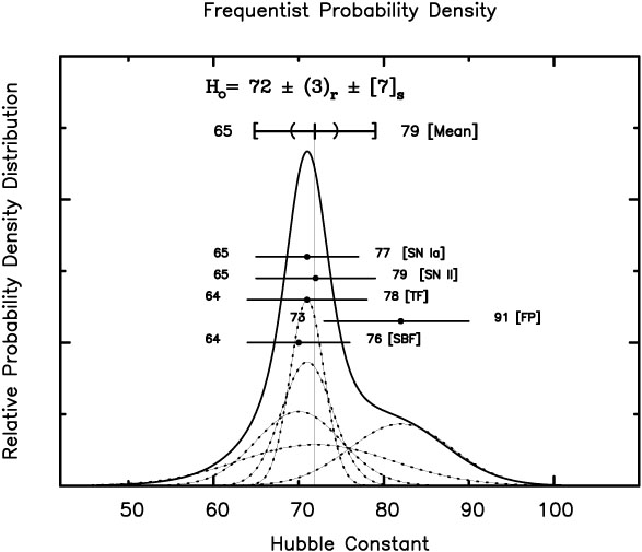
In Figure 3, we plot probability distributions for
the individual H0 determinations (see
Table 12),
each represented by a Gaussian of unit area, with a dispersion given
by their individual
values. The cumulative distribution is
given by the solid thick line. The frequentist solution, defined by
the median is H0 = 72 ± 3r (±
7s) km s-1 Mpc-1. The
random uncertainty is defined at the ±34% points of the
cumulative distribution. The systematic uncertainty is discussed
below. For our Bayesian analysis, we assume that the priors on
H0
and on the probability of any single measurement being correct are
uniform. In this case, we find H0 = 72 ± 2r
(± 7s)
km s-1 Mpc-1. The formal uncertainty on this
result is very small, and
simply reflects the fact that 4 of the values are clustered very
closely, while the uncertainties in the FP method are large.
Adjusting for the differences in calibration, these results are also
in excellent agreement with the weighting based on numerical
simulations of the errors by
Mould et
al. (2000a)
which yielded 71
± 6 km s-1 Mpc-1, similar to an earlier
frequentist and Bayesian analysis of Key Project data
(Madore et
al. 1999)
giving H0 = 72
± 5 ± 7 km s-1 Mpc-1, based on a smaller
subset of available Cepheid calibrators.
|
Figure 3. Values of H0 and their
uncertainties
for type Ia supernovae, the Tully-Fisher relation, the fundamental
plane, surface brightness fluctuations, and type II supernovae, all
calibrated by Cepheid variables. Each value is represented by a
Gaussian curve (joined solid dots) with unit area and a
1- |
As evident from Figure 3, the value of H0 based on the fundamental plane is an outlier. However, both the random and systematic errors for this method are larger than for the other methods, and hence, the contribution to the combined value of H0 is relatively low, whether the results are weighted by the random or systematic errors. We recall also from Table 1 and Section 6, that the calibration of the fundamental plane currently rests on the distances to only 3 clusters. If we weight the fundamental plane results factoring in the small numbers of calibrators and the observed variance of this method, then the fundamental plane has a weight that ranges from 5 to 8 times smaller than any of the other 4 methods, and results in a combined, metallicity-corrected value for H0 of 71 ± 4r km s-1 Mpc-1.
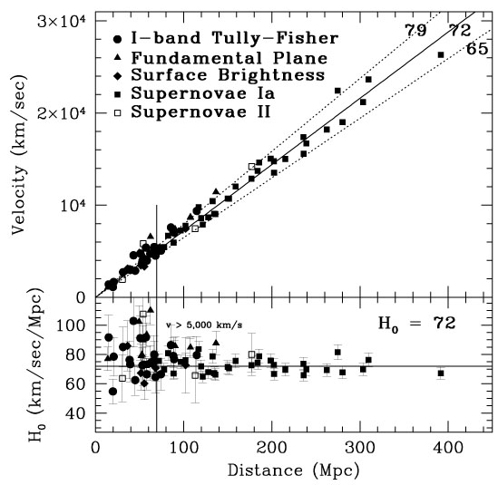
Figure 4 displays the results graphically in a composite Hubble diagram of velocity versus distance for Type Ia supernovae (solid squares), the Tully-Fisher relation (solid circles), surface-brightness fluctuations (solid diamonds), the fundamental plane (solid triangles), and Type II supernovae (open squares). In the bottom panel, the values of H0 are shown as a function of distance. The Cepheid distances have been corrected for metallicity, as given in Table 4. The Hubble line plotted in this figure has a slope of 72 km s-1 Mpc-1, and the adopted distance to the LMC is taken to be 50 kpc.
|
Figure 4. [Top panel]: A Hubble diagram of distance versus velocity for secondary distance indicators calibrated by Cepheids. Velocities in this plot are corrected for the nearby flow model of Mould et al. 2000a. The symbols are as follows: Type Ia supernovae - squares, Tully-Fisher clusters (I-band observations) - solid circles, Fundamental Plane clusters - triangles, surface brightness fluctuation galaxies - diamonds, Type II supernovae (open squares). A slope of H0 = 72 is shown, flanked by ±10% lines. Beyond 5,000 km/sec (indicated by the vertical line), both numerical simulations and observations suggest that the effects of peculiar motions are small. The Type Ia supernovae extend to about 30,000 km/sec and the Tully-Fisher and Fundamental Plane clusters extend to velocities of about 9,000 and 15,000 km/sec, respectively. However, the current limit for surface brightness fluctuations is about 5,000 km/sec. [Bottom panel:] Value of H0 as a function of distance. |