


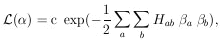
When M parameters are to be determined from a single experiment
containing N events, the error formulas of the preceding
section are applicable only in the rare case in which the errors
are uncorrelated.. Errors are uncorrelated only for
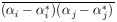 = 0 for all
cases with
i
= 0 for all
cases with
i  j. For the
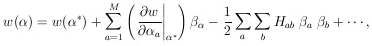
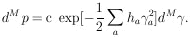
general case we Taylor-expand
w(
j. For the
general case we Taylor-expand
w( ) about
(*):
) about
(*):
|
where

|
and
| (9) |
The second term of the expansion vanishes because
ðw / ð = 0
are the equations for *
|
Neglecting the higher-order terms, we have
|
(an M-dimensional Gaussian surface). As before, our error
formulas depend on the approximation that
 () is
Gaussian-like in the region
i
() is
Gaussian-like in the region
i
 i*. As mentioned in
Section 4, if the
statistics are so poor that this is a poor approximation, then
one should merely present a plot of
(). (see Appendix IV).
i*. As mentioned in
Section 4, if the
statistics are so poor that this is a poor approximation, then
one should merely present a plot of
(). (see Appendix IV).
According to Eq. (9), H is a symmetric matrix. Let U be the unitary matrix that diagonalizes H:
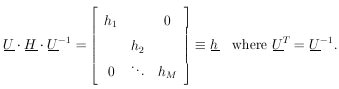
| (10) |
Let
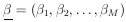 and
and
 . The
element of
probability in the
. The
element of
probability in the  -space is
|
Since
|U| = 1 is the Jacobian relating the volume elements
dM and
dM , we have
|
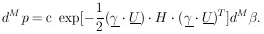
Now that the general M-dimensional Gaussian surface has been put in the form of the product of independent one-dimensional Gaussians we have

|
Then
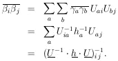
|
According to Eq. (10), H = U-1 . h . U, so that the final result is
| Maximum Likelihood Errors, M parameters (11) |
(A rule for calculating the inverse matrix H-1 is
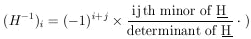
|
If we use the alternate notation V for the error matrix H-1, then whenever H appears, it must be replaced with V-1; i.e., the likelihood function is
| (11a) |
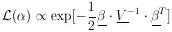
Example 2
Assume that the ranges of monoenergetic particles are
Gaussian-distributed with mean range
1 and straggling
coefficient
2 (the standard
deviation). N particles having ranges
x1,..., xN are observed. Find
1*,
2*, and their
errors . Then
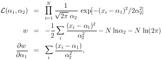
|
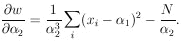
|
The maximum-likelihood solution is obtained by setting the above two equations equal to zero.
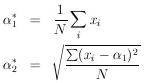
|
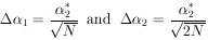
The reader may remember a standard-deviation formula in which N is replaced by (N - 1):
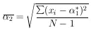
|
This is because in this case the most probable value,
2*, and
the mean,
 2 ,
do not occur at the same place. Mean
values of
such quantities are studied in Section 16.
The matrix H is
obtained by evaluating the following quantities at
1* and
2*:
2 ,
do not occur at the same place. Mean
values of
such quantities are studied in Section 16.
The matrix H is
obtained by evaluating the following quantities at
1* and
2*:
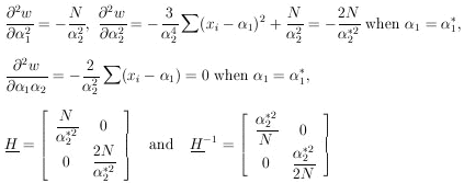
|
According to Eq. (11), the errors on
1 and
2 are the
square
roots of the diagonal elements of the error matrix, H-1:
| (this is sometimes
called the error of the error). |
We note that the error of the mean is
1/sqrt[N]
 where
=
2 is
the standard deviation. The error on the determination of
is
/sqrt[2N].
where
=
2 is
the standard deviation. The error on the determination of
is
/sqrt[2N].
Correlated Errors
The matrix
Vij  is
defined as the error matrix (also called the covariance matrix of
). In Eq. 11
we have shown that
V = H-1 where
Hij = - ð2 w /
(ði
ðj). The
diagonal elements of V are the variances of the
's. If all the
off-diagonal elements are zero, the errors in
are uncorrelated
as in Example 2. In this case contours of constant w plotted
in (1,
2) space would be
ellipses as shown in Fig. 2a. The
errors in 1 and
2 would be the
semi-major axes of the contour ellipse where w has dropped by
½ unit from its maximum-likelihood
value. Only in the case of uncorrelated errors is the rms error
is
defined as the error matrix (also called the covariance matrix of
). In Eq. 11
we have shown that
V = H-1 where
Hij = - ð2 w /
(ði
ðj). The
diagonal elements of V are the variances of the
's. If all the
off-diagonal elements are zero, the errors in
are uncorrelated
as in Example 2. In this case contours of constant w plotted
in (1,
2) space would be
ellipses as shown in Fig. 2a. The
errors in 1 and
2 would be the
semi-major axes of the contour ellipse where w has dropped by
½ unit from its maximum-likelihood
value. Only in the case of uncorrelated errors is the rms error
 j =
(Hjj)-½ and then there is no
need to perform a matrix inversion.
j =
(Hjj)-½ and then there is no
need to perform a matrix inversion.
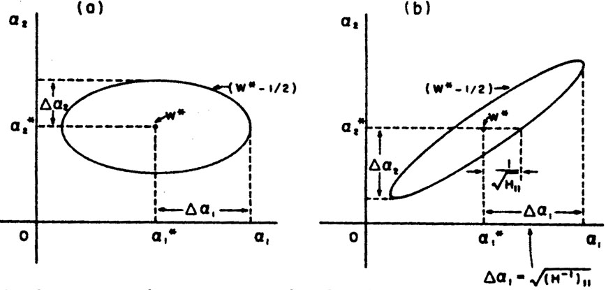
|
Figure 2. Contours of constant w as
a function of |
In the more common situation there will be one or more
off-diagonal elements to
H and the errors are correlated
(V has
off-diagonal elements). In this case (Fig. 2b)
the contour ellipses are inclined to the
1,
2 axes. The rms
spread of 1
is still 1 =
sqrt[V11], but it is the extreme limit of
the ellipse projected on the
1-axis. (The
ellipse "halfwidth" axis is
(H11)-½ which is smaller.) In cases
where Eq. 11 cannot be evaluated analytically, the
*'s can be found numerically and
the errors in can be found
by Plotting the ellipsoid where
w is 1/2 unit less than w * . The
extremums of this ellipsoid are
the rms error in the 's. One
should allow all the
j to change
freely and search for the maximum change in
i which makes
w = (w * - ½). This maximum
change in
i, is the
error in i and is
sqrt[V11].