4.2. Relationship to the Transfer Function

It is useful at this point to examine how the CCF is related to more fundamental quantities. Defined as a function of the continuous variable , the formal definition of the cross-correlation function is

(32)

If we use Eq. (21) to replace L(t) in this equation, we obtain

(33)

Comparing the inner integral with Eq. (32), we see that it is the cross-correlation of the continuum light curve with itself, i.e., the "autocorrelation function",

(34)

Thus, we see that the cross-correlation function is the convolution of the transfer function with the continuum autocorrelation function,

(35)

The centroid of the CCF is a usually quoted quantity,

(36)

which is related to the centroid of the transfer function

(37)

It is important to note that these two quantities are the same only in the limit where the light curves extend to infinity. Operationally, the centroid is computed using only points around the most significant peak, usually those points for which CCF() 0.8 r_peak, where r_peak is the maximum value of the CCF. Sometimes the location of the peak _peak (CCF(_peak) = r_peak) is the statistical quantity used.

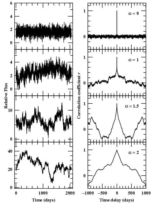
Cross-correlation does not necessarily give a clean and unambiguous measure of the relationship between two time series. In particular, the CCF is a convolution of the transfer function with the continuum ACF, so the CCF depends on the continuum behavior. To illustrate this, we show in Fig. 26 examples of light curves for various power-law PDSs (Eq. (7)) and the very different ACFs computed for each example.

Figure 26. The left-hand column shows artificial light curves generated with different power-law indices for the power-density spectra, P(f) f -. All light curves consist of 2048 points, normalized by setting Fvar = 0.3 (Eq. (2)). The right-hand column shows the autocorrelation functions for these light curves. Cases shown, top to bottom, are: (a) = 0. There is no correlation from one point to the next, as seen clearly in the ACF, which is essentially zero except at = 0. This is known as "white noise." (b) = 1. This is the power spectrum characteristic of a random walk; each continuum point now has some dependence on history. This case is sometimes called "flicker noise" (see Press 78 for further interesting discussion of this case). (c) = 1.5. This appears to be rather typical of AGN variability. (d) = 2. This power spectrum is characteristic of a superpositioning of independent events, which is often referred to as "shot noise."