3.4. Lacunarity

If in a fractal distribution, we count for each point the total number of neighbors within a ball of radius r, M(r), we can see that this quantity follows roughly a power-law

(5)

the exponent D is the so-called mass-radius dimension. Taking the average over all the points we get an estimate of the integral correlation function N( < r) = <M(r)>. In this section, we show how the correlation dimension alone is not enough to characterize the fractal structure.

The variability of the prefactor F in Eq. 5 can be used as a measure to distinguish between different fractal patterns having the same correlation dimension. This variability provides an indicator of the lacunarity. Several alternative quantitative measures have been proposed in the literature [40, 41, 42]. According to Ref. 43, we adopt the following numerical definition for the lacunarity, which is basically the second-order variability measure of the prefactor F in Eq. 5,

(6)

We first illustrate these measure on several two-dimensional point patterns.

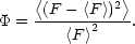
1. Mandelbrot [44] proposed an elegant fractal prescription to locate galaxies in space. It is the so-called Rayleigh-Lévy flight: galaxies are placed at the end points of a random walk with steps having isotropically random directions. The step length follows a power-law probability distribution function P(r > ) = (₀ / )^D for ₀ with D < 2, and P(r > ) = 1 for < ₀. Panel (a) in Fig. 6 shows a two-dimensional simulation with D = 1.5 and = 0.001 generated within a square with sidelength 1.
2. Soneira and Peebles [45] proposed a hierarchical fractal model to mimic the statistical properties of the Lick galaxy catalog. This model is built as follows: Within a sphere of radius R we place randomly spheres of radius R / with > 1. Now, in each of the new spheres, centers of smaller spheres with radius R/² are placed. This process is repeated until a given level L is reached. Galaxies are situated at the centers of the ^L spheres of the last level. 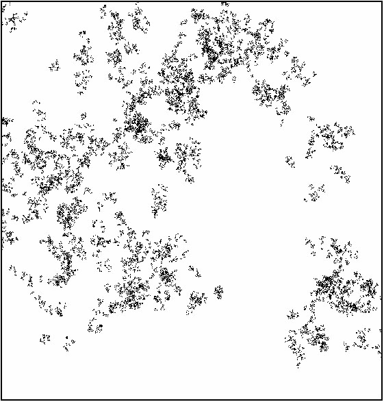The correlation dimension of this fractal clump is log() / log(). Panel (b) in Fig. 6 shows a two-dimensional simulation with = 2, = 1.587, and therefore D₂ = 1.5. Four clumps with L = 13 have been generated within a disc of diameter 1.
3. The next example is a multiplicative cascade process performed on the unit square [46]. First, the square is divided into four equal pieces. We assign a probability measure to each of the pieces randomly permuted from the set {p₁, p₂, p₃, p₄}. Each subsquare is divided again into four pieces, and again we attach a measure to each of the them by multiplying a p_i value randomly permuted by the value corresponding to its parent square. The process is repeated several times, and in each step the measure attached to each small square is the product of a new p_i value with all its ancestors. After L steps, we end with a mass distribution over a 2^L×2^L lattice. A point process is then generated placing randomly points within each pixel with probability proportional to its measure. Panels (c) and (d) in Fig. 6 show two realizations of this model, one being a simple fractal, panel (c), with p₁ = p₂ = p₃ = 1/3, and p₄ = 0 and the other one being a multifractal measure, panel (d), with p₁ = 0.4463, p₂ = 0.2537, p₃ = 0.3, and p₄ = 0. While for the first case D₂ = log 3 / log 2 1.58, for the multifractal measure the chosen values of p_i provide a dimensionality D₂ = 1.5.

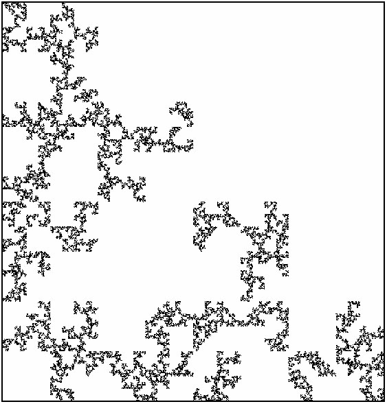
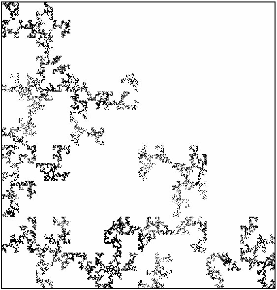
Figure 6. Panels (a)-(d) show different point patterns having similar correlation dimension: (a) Rayleigh-Lévy dust, (b) Soneira and Peebles model, (c) simple fractal distribution, (d) multifractal distribution. For all cases, the correlation integral follows a power law with similar exponent (panel (e) bottom). The central diagram in panel (e) shows the local correlation dimension calculated as the slope of the log-log linear regression within small portions of the scale range - the width of the sliding window is displayed by an arrow -. The lacunarity measure characterizing the textural properties of each point pattern is shown in the top diagram of panel (e).

The bottom panel of Fig. 6 shows the relation log N( < r) versus log r for the four examples. The power-law behavior N( < r) r^D₂ is clearly appreciated in the diagram, with scaling exponent D₂ 1.6 for all cases.

A more detailed analysis of the local correlation dimension is reported in the central diagram of panel (e), where we show how D₂ changes with the scale. In this case, D₂ has been calculated as the slope of the local linear regression fit to a small portion of the curve. This sliding window estimate of the local value of D₂ is very sensitive to any possible non fractal behavior that could not well be appreciated in the plot of log N( < r). The width of the sliding window used in the estimation is shown as an arrow in the bottom panel. We can see that in all the analyzed point patterns the empirical local correlation dimension oscillates around D₂ 1.6. It is therefore rather hard to find significative differences between the analyzed patterns through the function N( < r) or from D₂(r).

The differences, however, are revealed by the lacunarity measure (Eq. 6) which is shown in the top diagram of panel (e). The lacunarity curves (r), associated to each pattern, show clear differences between them providing us with a valuable information about the texture of each process.

The simple fractal model in panel (c) shows rather constant behavior of with the scale, displaying only very small oscillations around 0.1. By contrast, the multifractal set, being quite similar to the eye to the simple fractal, shows a completely different lacunarity curve, with a characteristic monotonic decreasing behavior from 0.7, at the smallest scales, to 0.2 at the larger scales. In this case the lacunarity is associated to the inhomogeneous distribution of the measure on the fractal support [40, 41] in which we can find highly populated regions (where the values of the measure are very large) together with other nearly empty locations (where the measure takes the lowest values). The lacunarity measure reveals the small scale heterogeneity of the multifractal set. Only at large scales the curve approaches that of the simple fractal pattern.

The lacunarity curve of the Soneira and Peebles model (panel (b)) is quite similar to that of the multifractal cascade model, with a decreasing behavior of with the scale. We can see in the plot that varies from 0.45 at the smallest scales to 0.08 at the largest analyzed distances. Because the different clumps overlap with each other, the set presents scale-dependent structure which cannot be discovered by analyzing the correlation function or the correlation dimension alone.

It is quite remarkable how the lacunarity curve of this model differs from the one corresponding to the Rayleigh-Lévy flight, although both spatial patterns seem quite similar to the eye. Within the first 2/3 of the analyzed scale range, the behavior of with the scale, for the Rayleigh-Lévy dust, is rather flat with oscillations around 0.4. It is, therefore, qualitatively similar to the behavior of the simple fractal pattern, although showing a higher value of and displaying oscillations with higher amplitude. The large-scale properties of finite regions of Rayleigh-Lévy dusts are extremely variable, and the rapid decrease of lacunarity at larger scales for the sample shown in panel (a) is typical only for dense subregions of a Rayleigh-Lévy flight.