


Although the diameter distribution leads to important conclusions, it would naturally be of greater interest to have access to the distribution of absolute magnitude. It seems possible to derive this distribution by an indirect procedure, without any knowledge of the magnitudes of the individual satellites.
In a previous investigation on the evolution of galaxies the writer (1964) has found pronounced relations between different galaxian characteristics. A study of the absolute pg magnitudes and log. absolute diameters, as listed in this paper, leads to the correlation diagram reproduced in Fig. 9. The diagram is based on 189 galaxies of types Sa-Sb-Sc, 36 of types E-So, 16 of type Ir I, and 5 of type Ir II, in all 246 objects. In order to facilitate comparisons with other results, the magnitudes have not been corrected for internal absorption, with the exception of the group Sa-Sb-Sc, for which differential absorption corrections have been applied. If the absorption-free magnitudes, as listed for the latter objects, are corrected by +1.0 magn. (Sa - Sb), or +0.7 magn. (Sc), they are reduced to a random orientation of the spirals with respect to the line of sight (the 5 Ir II objects have been treated as Sa-Sb spirals). The absolute magnitudes range from -9 and -11 (Leo I and Leo II, not included in the previous paper) to -21.5, and the absolute diameters from 0.7 to 50 kpc. The material thus covers the entire diameter range of the satellite population studied here.
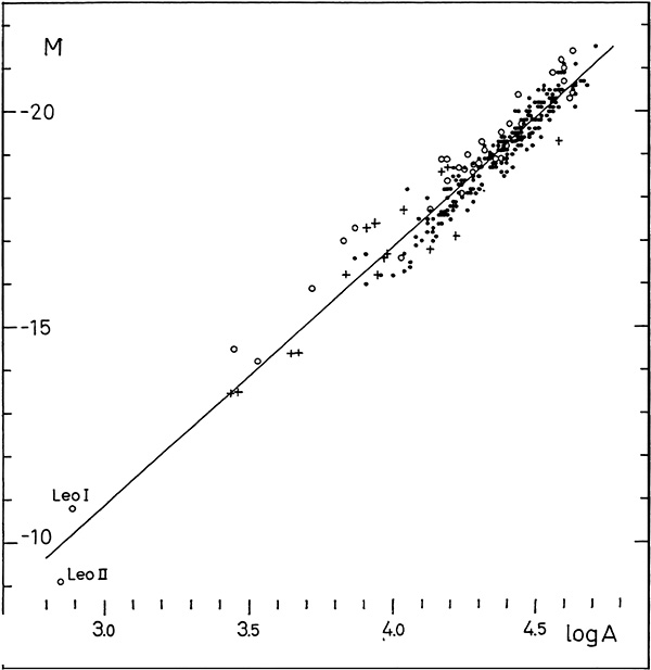 |
Figure 9. Relation between absolute pg magnitude and log. absolute major diameter (pc) as obtained from the Holmberg (1964) catalogue for galaxies of types E-So (open circles), Sa-Sb-Sc (filled circles), and Ir I (crosses). |
The relation is very pronounced, and apparently linear, the coefficient of correlation being -0.962 ± 0.005. The regression line reproduced in the figure has the equation:
 |
(1) |
The relation indicates that the surface magnitude gets fainter with decreasing size, the total variation being about two magnitudes from the largest galaxies to the smallest dwarfs. The dispersion of M around the regression line amounts to only 0.40 magn. On account of the accidental errors to be expected in the adopted distance moduli (and in the diameters) the final mean error in M, as derived from eq. (1), is estimated at 0.7 magn. It is of special interest that the different type groups of galaxies do not show any significant systematic deviations from the regression line; the only exception is the E-So group, with a deviation of about -0.3 magn.
By means of the above relation, the diameter distribution can be transformed to a distribution of absolute magnitude. In Fig. 8, the only change to be made is the replacement of the log. diameter scale by a magnitude scale. The absolute pg magnitude extends from -10.6, corresponding to the smallest diameter, up to -22.0, which seems to be the upper luminosity limit. The mean absolute magnitudes in the successive diameter classes are listed in the second column of Table 4.
The accuracy attained in the transformation process can be checked, for instance, by using the diameters and magnitudes available for the 160 central spiral systems. A comparison of the luminosity distribution, as derived from the diameters, with the same distribution obtained directly from the magnitudes indicates a very good agreement. A more conclusive check can be made by trying to determine the brighter end of the distribution curve in Fig. 8 directly from magnitudes. If we limit ourselves to luminosities higher than M = -16.5, an interval in which the disturbance from optical companions can be neglected, we find that magnitudes from the writer's catalogue are available for about two-thirds of the satellite population; magnitudes for the remainder can be obtained from other sources, in the first place, the catalogues by Zwicky et al. (1961, 1963, 1965, 1966, 1968). The distribution of the magnitudes for the 45 satellites brighter than M = -16.5 is given by the filled circles in Fig. 8. Considering the heterogeneity of the magnitude material, the points agree in a very satisfactory way with the adopted curve.