


In the calibration of the luminosity function of Fig. 10 the smoothed-out space density of galaxies brighter than M = -15.0 (outside the big clusters) has been assumed to be 0.17 per Mpc3. This figure represents a mean result derived from the analyses in this and the next section of the magnitudes, diameters, and redshifts of galaxies.
For comparison, it may be noted that the average space density in the 160 satellite groups investigated amounts to about 100 per Mpc3: The volume corresponding to each group is represented by a cylinder, pointing towards the observer, with a radius of 50 kpc and a length of about 600 kpc; the total volume corresponding to all the groups is equal to 0.75 Mpc3. The total number of satellites brighter than M = -15.0 is 74 (down to the limit M = -10.6 the total number is about 370).
In order to derive the space density from the magnitudes, it is necessary to have access to (a) the statistical distribution of the apparent magnitudes for a representative sample of galaxies, and (b) the distribution of the absolute magnitudes. As regards the former distribution, the curve previously derived by the writer (1958) may be used. The curve refers to all Shapley-Ames (1932) galaxies over the entire sky, with the exception of the galactic belt (gal. lat. -30° to +30°) and the Virgo cluster area. The Sh-A magnitudes have been individually reduced to the writer's photometric pg system by corrections that are mainly a function of the surface magnitudes of the objects; the mean error of the corrected magnitudes amounts to 0.3 magn. If the magnitudes are freed from the entire amount of galactic absorption by means of the Hubble (1934) cosecant-law, the statistical distribution is described by
 |
(3a) |
where N(m) is the total number of galaxies brighter than m in one square degree of of the sky. The inclination of the distribution line indicates a space density of galaxies that is independent of the distance.
The distribution function agrees comparatively well with the results obtained by Hubble (1934) from counts of galaxies on Mount Wilson plates. If Hubble's limiting magnitudes are corrected for redshift effect, and for systematic errors in the stellar magnitudes in the Selected Areas that were used for comparison, the constant term in the log. distribution will be approximately the same as that given in eq. (3 a). It may be pointed out in this connection that an evaluation of the effective limiting magnitude is a rather complicated problem, since the limit is no doubt a function of the galaxian type. A comparison with the distribution of galaxies, as derived by Shane and Wirtanen (1967) from the Lick Observatory counts of galaxies, has to await a definitive determination of the effective limiting magnitude.
According to well-known relations in stellar statistics, the space density D (1 Mpc3) of galaxies brighter than the absolute magnitude M' is obtained from the equation
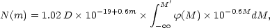 |
(3b) |
assuming that the density, and the luminosity function
 (M) ,
are independent of the distance. The integral can be determined by a
numerical integration based on the
curve of Fig. 10; it should be
noted that in this case
(M) is
the relative distribution
function. If the limiting magnitude M' is made equal to -15.0, the
integral has a value of 1.19 × 10¹¹.
(M) ,
are independent of the distance. The integral can be determined by a
numerical integration based on the
curve of Fig. 10; it should be
noted that in this case
(M) is
the relative distribution
function. If the limiting magnitude M' is made equal to -15.0, the
integral has a value of 1.19 × 10¹¹.
If eqs. (3 a) and (3 b) are combined, it is found that D = 0.16. Since the result is based on a Hubble parameter H = 80 km/sec per Mpc, it can be written in the following way:
 |
(3c) |
in order to correspond to any assumed value of H. The result refers to a limiting pg magnitude M' = -15.0 but can easily be reduced to other values of M' by means of the luminosity curve of Fig. 10 (and Fig. 8).
The statistical distribution of the apparent diameters of galaxies needed for the determination of space density from diameters can be derived from the present material. Measures of major diameters are available for over 3000 galaxies in the survey areas and comparison areas. The homogeneity of this material has been discussed in sect. 5; except for a certain decrease in the number of very small galaxies, presumably a redshift effect, the distribution of the diameters appears to be consistent with the assumption of a space density independent of the distance. If the smallest diameters are left out, the distribution of the log. diameters (as reduced to the writer's photometric diameter system; cf. sect. 10) of the galaxies in all the survey areas and comparison areas is described by the relation
 |
(4a) |
where N(log a) is the total number of galaxies in one square degree having diameters larger than a (min. of arc). The space density is in this case obtained from the equation
 |
(4b) |
where (log
A) is the relative distribution of the
log. absolute major diameters (pc),
which is assumed to be independent of the distance. The space density
refers to all galaxies having absolute diameters larger than the limit
A'. If the latter diameter
is made equal to 5000 pc, corresponding approximately to an absolute
magnitude of
-15.0 (cf. eq. 1 ), a numerical integration based on the curve of
Fig. 8 gives a value
for the integral of 4.5 × 10¹². Accordingly, the space
density is equal to 0.15 per Mpc3.
Although it is difficult to define exactly the absolute diameter that
would correspond to the above limiting magnitude M' = -15.0, it is
satisfactory to note that the space density found from the diameters is
nearly the same as the density derived from the magnitudes.