7.2. Inflationary predictions

The most commonly-discussed mechanism for generating the inhomogeneities that act as the source for T / T is inflation. Of course, CMB anisotropies were calculated in largely the modern way well before inflation was ever considered, by Peebles & Yu (1970). The standard approach involves super-horizon fluctuations, which must be generated by some acausal process. Inflation achieves this - but we cannot claim that detection of super-horizon modes amounts to a proof of inflation. Rather, we need some more characteristic signature of the specific process used by inflation: amplified quantum fluctuations (see e.g. chapter 11 of Peacock 1999 or Liddle & Lyth 2000 for details).

In the simplest models, inflation is driven by a scalar field , with a potential V(). As well as the characteristic energy density of inflation, V, this can be characterized by two parameters, & , which are dimensionless versions of the first and second derivatives of V with respect to . In these terms, the inflationary predictions for the perturbation index is

(142)

Since inflation continues while & are small, some tilt is expected (| n - 1| ~ 0.01 to 0.05 in simple models).

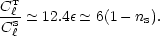
The critical ingredient for testing inflation by making further predictions is the possibility that, in addition to scalar modes, the CMB could also be affected by gravitational waves (following the original insight of Starobinsky 1985). The relative amplitude of tensor and scalar contributions depended on the inflationary parameter alone:

(143)

The second relation to the tilt is less general, as it assumes a polynomial-like potential, so that is related to . For example, V = ⁴ implies n_S 0.95 and C^T / C^S 0.3. To be safe, we need one further observation, and this is potentially provided by the spectrum of C^T. Suppose we write separate power-law index definitions for the scalar and tensor anisotropies:

(144)

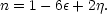
For the scalar spectrum, we had n_S = n = 1 - 6 + 2; for the tensors, n_T = 1 - 2 [although different definitions of n_T exist; the convention here is that n = 1 always corresponds to a constant ²()]. Thus, a knowledge of n_S, n_T and the scalar-to-tensor ratio would overdetermine the model and allow a genuine test of inflation.