11.7. HIGH-RESOLUTION MAPS

11.7.1. Observations of M33 with the Cambridge Half-Mile Telescope

a) Observations

The highest resolution observations of an external galaxy so far made using aperture synthesis techniques are those of M33, made with the Cambridge Half-Mile Telescope (Wright, Warner, and Baldwin, 1972). This telescope consists of two 9-m paraboloids on an east-west baseline and was designed as an aperture synthesis instrument for observing extended objects. The observations of M33 have an angular resolution of 1.5 minutes are in RA and 3 minutes arc in declination, equivalent to a 300 × 600 pc area at the distance of M33 (690 kpc). (This compares with a linear resolution of 210 pc in the Magellanic Clouds using the Parkes 210-foot telescope.) The velocity resolution of these data is 39 km sec^-1, commensurate with the range of velocities expected within a 300 × 600 pc area over most of the galaxy. Observations were made at 59 interferometer baselines with telescope separations at 6m intervals to a maximum of 360m. The full baseline (720 m, a half-mile) was not used for reasons of sensitivity, as discussed in the previous section. The data were obtained using an analogue cross-correlation receiver and were processed much as described in the previous section. The basic data are in the form of nine maps of the HI distribution at 26 km sec^-1 intervals. These nine maps cover the range of velocities found in the neutral hydrogen of M33.

b) Integrated HI Brightness Distribution

For these observations the half-width of a velocity channel is larger than the velocity interval between the channels, and a simple addition of these nine maps suffices to construct a map of the integrated hydrogen distribution in M33 (Figure 11.4). This map is of the surface brightness temperature of the hydrogen line integrated over the line profile.

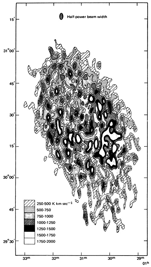Figure 11.4. Integrated HI brightness in M33 to an angular resolution of 1.5 × 3 minutes arc. [Wright et al., Monthly Notices Roy. Astron. Soc. (1972) 155:337.]

If the galaxy is everywhere optically thin to the line radiation, then the map also represents the distribution of the HI surface density projected along the line of sight. The peak brightness temperature observed is 50° K but the distribution is in places unresolved in both angle and velocity so that the true brightness temperature may exceed 100° K and the line radiation may not be optically thin. Where the radiation is not optically thin, the brightness temperature gives only a lower limit to the surface density. There is no direct evidence of optically thick HI from absorption of continuum sources lying behind or in the disk of M33, and we can adopt as a working hypothesis that the line radiation is optically thin, so that the map of the integrated brightness temperature is also a map of the HI surface density.

c) Large-Scale Structure

The large-scale structure of the hydrogen distribution may be obtained with a higher signal-to-noise ratio on a lower-resolution map (which may be obtained in aperture synthesis observations by simply not including data from the larger interferometer spacings in the Fourier transform). A low-resolution map generated from the above data agrees well with the map obtained by Gordon (1971) with the NRAO 300-foot telescope and described in Section 11.4. Figure 11.5 is an integration in elliptical rings (circular in the galaxy plane) of the brightness temperatures of Figure 11.4, and shows that the average radial distribution is a plateau with a very sharp cut-off at the edges. The radial distribution in Figure 11.5 is not in good agreement with the suggestion by Roberts (1967) that the HI has a ring distribution as in M31. The average projected surface density is 3 × 10²¹ atoms cm^-2, or 1.7 × 10²¹ cm^-2 viewed normal to the plane of the galaxy. The sharp fall in density at the edges of the galaxy could be due to ionization by an inter-galactic flux of UV photons, as discussed by Sunyaev (1969). An alternative explanation is that the sharp gradients at the edges of the galaxy are associated with the warping of the plane of the HI disk indicated by the wings of the galaxy. A hat-brim model is envisaged with an increasing inclination of the plane of the galaxy to the line of sight along the edges of the galaxy at the ends of the minor axis.

There is a marked asymmetry in the HI distribution with a massive HI complex in the south-preceding quadrant of the galaxy.

Figure 11.5. Integration in circular rings in the plane of M33 of the integrated brightness distribution. [Wright et al., Monthly Notices Roy. Astron. Soc. (1972) 155:337.]

The HI distribution is broken up into a large number of concentrations only partially resolved by the 1.5 × 3.0 minute arc beam. These concentrations have a typical peak surface density of 2.7 × 10²¹ cm^-2 and a space density of ~ 1 to 2 atom cm^-3. They perhaps resemble the complexes discussed by McGee (1964) in the spiral arms of our galaxy, having sizes 500 to 2500 pc and densities 0.5 cm^-3, and those in the Large Magellanic Cloud having mean diameter 600 pc and density 1 cm^-3. A spiral arm structure can be seen in the inner regions of the galaxy and is most evident in the trough running south from the galactic center (Figure 11.4). A best-fitting logarithmic spiral structure agrees with the optical spiral arms and the measured ratio of the average projected HI density in the arm and interarm regions is between 2 or 3 to 1. The troughs between HI concentrations are barely resolved by the beam, and the true density ratio may be as large as 6 to 1. An infinite contrast ratio is, however, ruled out by these observations.

e) Comparison with Optical Features

The extent of the HI distribution corresponds well with that of a well-exposed blue-print of the galaxy and the major and minor axis widths are close to the 83 × 53 minute arc given for the optical size by Holmberg (1958).

Figure 11.6 shows a superposition of the HI peaks onto a plate taken through a narrow-band red filter. It can be seen that the Mapping Neutral Hydrogen in External Galaxies HI concentrations follow the line of the optical spiral arms well in the south of the galaxy. The correlation is not so clear, and there are no strong HI concentrations on the northern spiral arm between the nucleus and NGC 604, where there is again a large concentration of HI. The contrast of the spiral arms is better in the composite HI + HII distribution in Figure 11.6 than in either the HI or HII regions separately, which indicates that the HI and HII are in some sense complementary.

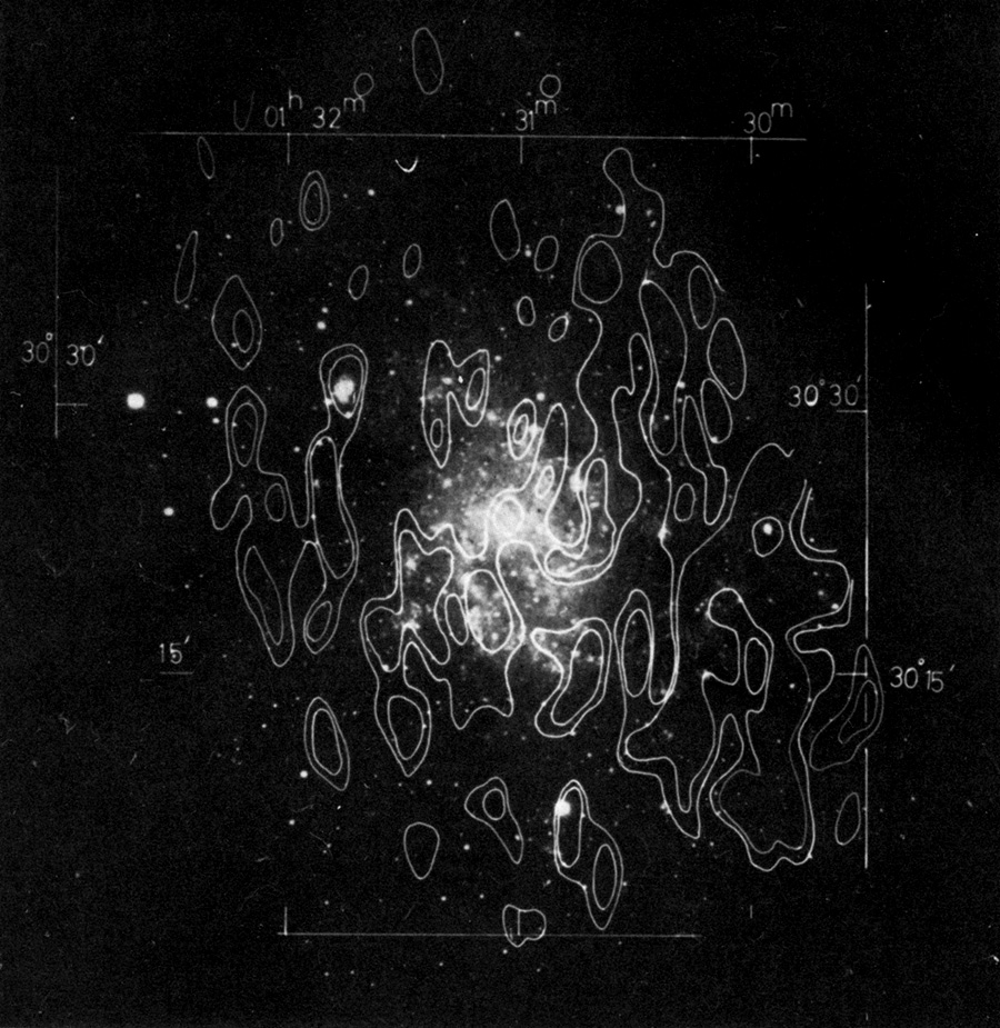Figure 11.6. Superposition of the peaks of the HI distribution of M33 on a red print showing mainly HII regions.

The isovelocity contours (Figure 11.7) conform well to the pattern expected for a rotating galaxy and the rotation curve measured along the major axis is shown in Figure 11.8. The total mass can be derived by fitting a model rotation curve. The observed rotation curve has been fitted to three different types of rotation curve: a Brandt rotation curve with n = 1.0, a curve corresponding to an exponential distribution of mass (as discussed by Freeman, 1970), and an eighth-order polynomial. In all three cases the fitted curves agree with the observed rotation curve within 3 km sec^-1, and it will clearly be difficult to distinguish among them. The distributions of mass with radius deduced from these three fitted rotation curves are very similar within 20 minutes arc radius but diverge outside this radius. Using a Brandt curve with R_max = 30 minutes arc, V_max = 100 km sec^-1, and n = 1.0 gives a mass within 45 minutes arc of 1.7 × 10¹⁰ M. The HI content is then some 9%, typical for an Sc galaxy. Because of the very flat rotation curve, the total mass of the galaxy extrapolated beyond the observed rotation curve is some 5 × 10¹⁰ M), but this does not have much meaning.

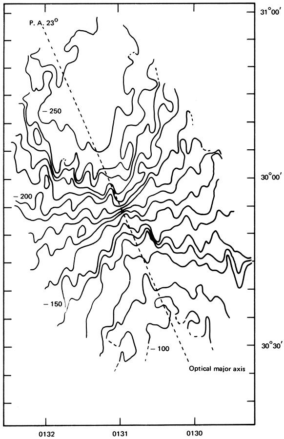Figure 11.7. Isovelocity contours in M33 drawn at intervals of 10 km sec-1.

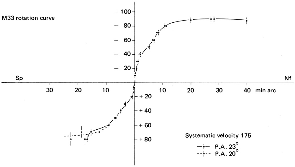Figure 11.8. Rotation curve measured along the major axis of M33. The rotation velocities uncorrected for inclination are referred to a heliocentric systematic velocity of -175 km sec-1.

It is clear from Figure 11.7 that there are local departures of the isovelocities from circular motion which exceed the noise level. It is essential, however, to consider the effect of beam averaging. A superposition of Figure 11.4 and Figure 11.7 shows that the deformations in the isovelocity contours often correspond to their crossing between HI peaks. The velocity in the interarm region is a beam average of the velocities of all HI concentrations within the beam at that time, and we may consequently discount many of the departures from smooth isovelocities. Some of the departures are real, however, and local peculiar velocities can be 20 to 30 km sec^-1.

The line-of-sight velocity due to the rotation of the galaxy may be computed by selecting values for the rotation center, position angle, inclination, and rotation curve of the galaxy. If this model velocity field is subtracted from the observed velocity field, errors in the parameters selected show up in the residual velocity field with characteristic symmetries and enable best values for the rotation parameters to be determined. The residual velocity field may then be examined for systematic streaming motions predicted by the density wave theory of spiral arms. From the present observations of M33 it appears that such streaming motions are less than about 5 km sec^-1.

h) Comparison of Neutral and Ionized Hydrogen Velocities

In Figure 11.9 are plotted the velocities of the large HII regions measured by Mayall and Aller (1942) against the HI velocity at the HII region position. Because of the relatively large beamwidth (1.5 × 3 minutes arc), the HI Velocities are best regarded as an average velocity of HI in the vicinity of the HII region. The HII region velocities are local velocities of ionized gas within the HII region. The straight line has a slope of 1, showing that there is no systematic difference between the velocities of neutral and ionized gas. The vertical scatter in Figure 11.9 shows that, the velocity of an HII region can differ by 20 to 30 km sec^-1 from that of the neutral gas. Indeed, measurements within a single HII region can differ by the same magnitude. Estimates of the mass of gas in large HII regions, e.g., in 30 Doradus in the LMC (Faulkner, 1967) and in NGC 604 in M33 (Wright, 1971b), show that velocity dispersions of this magnitude will disperse the HII region in 10⁷ years.

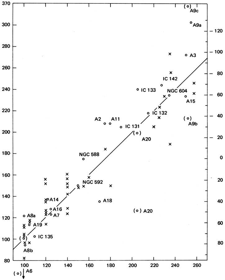Figure 11.9. Velocities of HII regions (ordinate) plotted against the neutral hydrogen velocity at the position of the HII region. Open circles, o, are HII regions measured by Mayall and Aller (1942) with velocities by Brandt (1965); (o) velocities are measured by Mayall and Aller; (x) velocities are measured by Carranza et al. (1968). The left ordinate and abscissa scale are heliocentric, and the right ordinate is with respect to a systematic velocity of -175 km sec-1. The line has a slope of 1.