


Since the COBE DMR detection of CMB anisotropy (Smoot et al., 1992), there have been over thirty additional measurements of anisotropy on angular scales ranging from 7° to 0.°3, and upper limits have been set on smaller scales.
The COBE DMR observations
were pixelized into a skymap, from which it is possible to analyze any
particular multipole within the resolution of the DMR.
Current small angular scale
CMB anisotropy observations are insensitive to both high
 and
low
multipoles because they cannot measure features smaller than their
resolution and are insensitive to features larger than the
size of the patch of sky observed.
The next satellite mission, NASA's Microwave Anisotropy Probe
(MAP), is scheduled for launch in Fall 2000
and will map angular scales down to 0.°2 with high precision over
most of the sky. An even more precise satellite, ESA's Planck, is
scheduled for launch in 2007. Because COBE observed such large angles,
the DMR data can only
constrain the amplitude A and index n of
the primordial power spectrum in wave number k,
Pp(k) = Akn, and
these constraints are not tight enough
to rule out very many classes of cosmological models.
and
low
multipoles because they cannot measure features smaller than their
resolution and are insensitive to features larger than the
size of the patch of sky observed.
The next satellite mission, NASA's Microwave Anisotropy Probe
(MAP), is scheduled for launch in Fall 2000
and will map angular scales down to 0.°2 with high precision over
most of the sky. An even more precise satellite, ESA's Planck, is
scheduled for launch in 2007. Because COBE observed such large angles,
the DMR data can only
constrain the amplitude A and index n of
the primordial power spectrum in wave number k,
Pp(k) = Akn, and
these constraints are not tight enough
to rule out very many classes of cosmological models.
Until the next satellite is flown, the promise of microwave background anisotropy measurements to measure cosmological parameters rests with a series of ground-based and balloon-borne anisotropy instruments which have already published results (shown in Figure 4) or will report results in the next few years (MAXIMA, BOOMERANG, TOPHAT, ACE, MAT, VSA, CBI, DASI, see Lee et al., 1999 and Halpern & Scott, 1999). Because they are not satellites, these instruments face the problems of shorter observing times and less sky coverage, although significant progress has been made in those areas. They fall into three categories: high-altitude balloons, interferometers, and other ground-based instruments. Past, present, and future balloon-borne instruments are FIRS, MAX, MSAM, ARGO, BAM, MAXIMA, QMAP, HACME, BOOMERANG, TOPHAT, and ACE. Ground-based interferometers include CAT, JBIAC, SUZIE, BIMA, ATCA, VLA, VSA, CBI, and DASI, and other ground-based instruments are TENERIFE, SP, PYTHON, SK, OVRO/RING, VIPER, MAT/TOCO, IACB, and WD. Taken as a whole, they have the potential to yield very useful measurements of the radiation power spectrum of the CMB on degree and subdegree scales. Ground-based non-interferometers have to discard a large fraction of data and undergo careful further data reduction to eliminate atmospheric contamination. Balloon-based instruments need to keep a careful record of their pointing to reconstruct it during data analysis. Interferometers may be the most promising technique at present but they are the least developed, and most instruments are at radio frequencies and have very narrow frequency coverage, making foreground contamination a major concern. In order to use small-scale CMB anisotropy measurements to constrain cosmological models we need to be confident of their validity and to trust the error bars. This will allow us to discard badly contaminated data and to give greater weight to the more precise measurements in fitting models. Correlated noise is a great concern for instruments which lack a rapid chopping because the 1/f noise causes correlations on scales larger than the beam in a way that can easily mimic CMB anisotropies. Additional issues are sample variance caused by the combination of cosmic variance and limited sky coverage and foreground contamination.
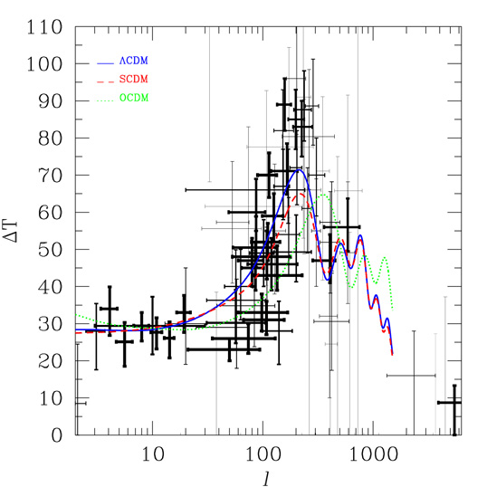 |
Figure 4. Compilation of CMB Anisotropy
observations. Vertical error bars represent
1 |
| Instrument |  T (µK)
 |
+
1 (µK) (µK) |
-
1(µK) |
eff |
min |
max |
1 cal. |
ref. |
| COBE1 | 8.5 | 16.0 | 8.5 | 2.1 | 2 | 2.5 | 0.7 | 1 |
| COBE2 | 28.0 | 7.4 | 10.4 | 3.1 | 2.5 | 3.7 | 0.7 | 1 |
| COBE3 | 34.0 | 5.9 | 7.2 | 4.1 | 3.4 | 4.8 | 0.7 | 1 |
| COBE4 | 25.1 | 5.2 | 6.6 | 5.6 | 4.7 | 6.6 | 0.7 | 1 |
| COBE5 | 29.4 | 3.6 | 4.1 | 8.0 | 6.8 | 9.3 | 0.7 | 1 |
| COBE6 | 27.7 | 3.9 | 4.5 | 10.9 | 9.7 | 12.2 | 0.7 | 1 |
| COBE7 | 26.1 | 4.4 | 5.3 | 14.3 | 12.8 | 15.7 | 0.7 | 1 |
| COBE8 | 33.0 | 4.6 | 5.4 | 19.4 | 16.6 | 22.1 | 0.7 | 1 |
| FIRS | 29.4 | 7.8 | 7.7 | 10 | 3 | 30 | -a | 2 |
| TENERIFE | 30 | 15 | 11 | 20 | 13 | 31 | -a | 3 |
| IACB1 | 111.9 | 49.1 | 43.7 | 33 | 20 | 57 | 20 | 4 |
| IACB2 | 57.3 | 16.4 | 16.4 | 53 | 38 | 75 | 20 | 4 |
| SP91 | 30.2 | 8.9 | 5.5 | 57 | 31 | 106 | 15 | 5 |
| SP94 | 36.3 | 13.6 | 6.1 | 57 | 31 | 106 | 15 | 5 |
| BAM | 55.6 | 27.4 | 9.8 | 74 | 28 | 97 | 20 | 6 |
| ARGO94 | 33 | 5 | 5 | 98 | 60 | 168 | 5 | 7 |
| ARGO96 | 48 | 7 | 6 | 109 | 53 | 179 | 10 | 8 |
| JBIAC | 43 | 13 | 12 | 109 | 90 | 128 | 6.6 | 9 |
| QMAP(Ka1) | 47.0 | 6 | 7 | 80 | 60 | 101 | 12 | 10 |
| QMAP(Ka2) | 59.0 | 6 | 7 | 126 | 99 | 153 | 12 | 10 |
| QMAP(Q) | 52.0 | 5 | 5 | 111 | 79 | 143 | 12 | 10 |
| MAX234 | 46 | 7 | 7 | 120 | 73 | 205 | 10 | 11 |
| MAX5 | 43 | 8 | 4 | 135 | 81 | 227 | 10 | 12 |
| MSAMI | 34.8 | 15 | 11 | 84 | 39 | 130 | 5 | 13 |
| MSAMII | 49.3 | 10 | 8 | 201 | 131 | 283 | 5 | 13 |
| MSAMIII | 47.0 | 7 | 6 | 407 | 284 | 453 | 5 | 13 |
| PYTHON123 | 60 | 9 | 5 | 87 | 49 | 105 | 20 | 14 |
| PYTHON3S | 66 | 11 | 9 | 170 | 120 | 239 | 20 | 14 |
| PYTHONV1 | 23 | 3 | 3 | 50 | 21 | 94 | 17b | 15 |
| PYTHONV2 | 26 | 4 | 4 | 74 | 35 | 130 | 17 | 15 |
| PYTHONV3 | 31 | 5 | 4 | 108 | 67 | 157 | 17 | 15 |
| PYTHONV4 | 28 | 8 | 9 | 140 | 99 | 185 | 17 | 15 |
| PYTHONV5 | 54 | 10 | 11 | 172 | 132 | 215 | 17 | 15 |
| PYTHONV6 | 96 | 15 | 15 | 203 | 164 | 244 | 17 | 15 |
| PYTHONV7 | 91 | 32 | 38 | 233 | 195 | 273 | 17 | 15 |
| PYTHONV8 | 0 | 91 | 0 | 264 | 227 | 303 | 17 | 15 |
| SK1c | 50.5 | 8.4 | 5.3 | 87 | 58 | 126 | 11 | 16 |
| SK2 | 71.1 | 7.4 | 6.3 | 166 | 123 | 196 | 11 | 16 |
| SK3 | 87.6 | 10.5 | 8.4 | 237 | 196 | 266 | 11 | 16 |
| SK4 | 88.6 | 12.6 | 10.5 | 286 | 248 | 310 | 11 | 16 |
| SK5 | 71.1 | 20.0 | 29.4 | 349 | 308 | 393 | 11 | 16 |
| TOCO971 | 40 | 10 | 9 | 63 | 45 | 81 | 10 | 17 |
| TOCO972 | 45 | 7 | 6 | 86 | 64 | 102 | 10 | 17 |
| TOCO973 | 70 | 6 | 6 | 114 | 90 | 134 | 10 | 17 |
| TOCO974 | 89 | 7 | 7 | 158 | 135 | 180 | 10 | 17 |
| TOCO975 | 85 | 8 | 8 | 199 | 170 | 237 | 10 | 17 |
| TOCO981 | 55 | 18 | 17 | 128 | 102 | 161 | 8 | 18 |
| TOCO982 | 82 | 11 | 11 | 152 | 126 | 190 | 8 | 18 |
| TOCO983 | 83 | 7 | 8 | 226 | 189 | 282 | 8 | 18 |
| TOCO984 | 70 | 10 | 11 | 306 | 262 | 365 | 8 | 18 |
| TOCO985 | 24.5 | 26.5 | 24.5 | 409 | 367 | 474 | 8 | 18 |
| VIPER1 | 61.6 | 31.1 | 21.3 | 108 | 30 | 229 | 8 | 19 |
| VIPER2 | 77.6 | 26.8 | 19.1 | 173 | 72 | 287 | 8 | 19 |
| VIPER3 | 66.0 | 24.4 | 17.2 | 237 | 126 | 336 | 8 | 19 |
| VIPER4 | 80.4 | 18.0 | 14.2 | 263 | 150 | 448 | 8 | 19 |
| VIPER5 | 30.6 | 13.6 | 13.2 | 422 | 291 | 604 | 8 | 19 |
| VIPER6 | 65.8 | 25.7 | 24.9 | 589 | 448 | 796 | 8 | 19 |
| BOOM971 | 29 | 13 | 11 | 58 | 25 | 75 | 8.1 | 20 |
| BOOM972 | 49 | 9 | 9 | 102 | 76 | 125 | 8.1 | 20 |
| BOOM973 | 67 | 10 | 9 | 153 | 126 | 175 | 8.1 | 20 |
| BOOM974 | 72 | 10 | 10 | 204 | 176 | 225 | 8.1 | 20 |
| BOOM975 | 61 | 11 | 12 | 255 | 226 | 275 | 8.1 | 20 |
| BOOM976 | 55 | 14 | 15 | 305 | 276 | 325 | 8.1 | 20 |
| BOOM977 | 32 | 13 | 22 | 403 | 326 | 475 | 8.1 | 20 |
| BOOM978 | 0 | 130 | 0 | 729 | 476 | 1125 | 8.1 | 20 |
| CAT96I | 51.9 | 13.7 | 13.7 | 410 | 330 | 500 | 10 | 21 |
| CAT96II | 49.1 | 19.1 | 13.7 | 590 | 500 | 680 | 10 | 21 |
| CAT99I | 57.3 | 10.9 | 13.7 | 422 | 330 | 500 | 10 | 22 |
| CAT99II | 0. | 54.6 | 0. | 615 | 500 | 680 | 10 | 22 |
| OVRO/RING | 56.0 | 7.7 | 6.5 | 589 | 361 | 756 | 4.3 | 23 |
| HACME | 0. | 38.5 | 0. | 38 | 18 | 63 | -a | 29 |
| WD | 0. | 75.0 | 0. | 477 | 297 | 825 | 30 | 24 |
| SuZIE | 16 | 12 | 16 | 2340 | 1330 | 3070 | 8 | 25 |
| VLA | 0. | 27.3 | 0. | 3677 | 2090 | 5761 | -a | 26 |
| ATCA | 0. | 37.2 | 0. | 4520 | 3500 | 5780 | -a | 27 |
| BIMA | 8.7 | 4.6 | 8.7 | 5470 | 3900 | 7900 | -a | 28 |
REFERENCES: 1-
Kogut et
al. (1996a);
Tegmark &
Hamilton (1997)
2-
Ganga et
al. (1994)
3-
Gutierrez et
al. (1999)
4-
Femenia et
al. (1998)
5-
Ganga et
al. (1997b);
Gundersen et
al. (1995)
6-
Tucker et
al. (1997)
7-
Ratra et
al. (1999)
8-
Masi et al. (1996)
9-
Dicker et
al. (1999)
10-
De Oliveira-Costa
et al. (1998)
11-
Clapp et
al. (1994);
Tanaka et
al. (1996)
12-
Ganga et
al. (1998)
13-
Wilson et
al. (1999)
14-
Platt et
al. (1997)
15-
Coble et
al. (1999)
16-
Netterfield
et al. (1997)
17-
Torbet et
al. (1999)
18-
Miller et
al. (1999)
19-
Peterson et
al. (1999)
20-
Mauskopf et
al. (1999)
21-
Scott et
al. (1996)
22-
Baker et
al. (1999)
23-
Leitch et
al. (1998)
24-
Ratra et
al. (1998)
25-
Church et
al. (1997);
Ganga et
al. (1997a)
26-
Partridge et
al. (1997)
27-
Subrahmanyan
et al. (1993)
28-
Holzapfel et
al. (1999)
29-
Staren et
al. (1999)
|
||||||||
Figure 4
shows our compilation of CMB anisotropy observations without
adding any theoretical curves to bias the eye
2.
It is clear that a straight line is a poor but not implausible fit to
the data. There is a clear rise around
= 100 and then a
drop by = 1000. This is not
yet good enough to give a clear determination of the curvature of the
universe, let alone fit several cosmological parameters.
However, the current data prefer
adiabatic structure formation models over isocurvature models
(Gawiser &
Silk, 1998).
If analysis is restricted to adiabatic CDM models, a value of the total
density near critical is preferred
(Dodelson &
Knox, 1999).
The sensitivity of these instruments to various multipoles is called
their window function. These window functions
are important in analyzing anisotropy measurements because
the small-scale experiments do not measure enough of the sky to produce
skymaps like COBE. Rather they yield a few
"band-power" measurements of rms temperature anisotropy which reflect
a convolution over the range of multipoles contained in the window
function of each band. Some instruments can produce limited skymaps
(White & Bunn,
1995).
The window function W shows
how the total power observed is sensitive to the anisotropy on
the sky as a function of angular scale:
 |
(13) |
where the COBE normalization is
T = 27.9
µK and TCMB = 2.73 K
(Bennett et
al., 1996).
This allows the observations of broad-band
power to be reported as observations of
T, and
knowing the window function of an instrument one can turn the predicted
C spectrum
of a model into the corresponding prediction for
T.
This "band-power" measurement
is based on the standard definition that for a "flat" power spectrum,
T =
(( + 1)
C)1/2 TCMB /
(2 ) (flat actually means that
( + 1)
C is constant).
) (flat actually means that
( + 1)
C is constant).
The autocorrelation function for measured temperature anisotropies is a convolution of the true expectation values for the anisotropies and the window function. Thus we have (White & Srednicki, 1995)
 |
(14) |
where the symmetric beam shape that is typically assumed makes
W a
function of separation angle only. In general, the window function
results from a combination of the directional response of the antenna,
the beam position as a function of time, and the weighting of each
part of the beam trajectory in producing a temperature measurement
(White &
Srednicki, 1995).
Strictly speaking, W is the diagonal part of a filter function
W
' that
reflects the coupling of
various multipoles due to the non-orthogonality of the spherical
harmonics on a cut sky and the observing strategy of the instrument
(Knox, 1999).
It is standard to assume a Gaussian beam response of width
,
leading to a window function
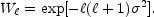 |
(15) |
The low-
cutoff introduced by a 2-beam differencing setup comes from the window
function
(White et al.,
1994)
 |
(16) |
4.2. Sample and Cosmic Variance
The multipoles C can be related to the expected
value of the spherical harmonic coefficients by
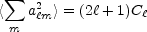 |
(17) |
since there are
(2 + 1)
am for each
and each has
an expected autocorrelation of C. In a theory
such as inflation,
the temperature fluctuations follow a Gaussian distribution about
these expected ensemble averages. This makes the
am Gaussian random variables, resulting in a
 22+1
distribution for
22+1
distribution for
 m
am2. The width of this distribution leads
to a cosmic variance in the estimated
C of
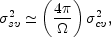
cv2
= ( + 1/2)-1/2
C, which
is much greater for small
than for large (unless
C is rising in a
manner highly inconsistent with theoretical expectations). So, although
cosmic variance is an unavoidable source of error for anisotropy
measurements, it is much less of a problem for small scales
than for COBE.
m
am2. The width of this distribution leads
to a cosmic variance in the estimated
C of
cv2
= ( + 1/2)-1/2
C, which
is much greater for small
than for large (unless
C is rising in a
manner highly inconsistent with theoretical expectations). So, although
cosmic variance is an unavoidable source of error for anisotropy
measurements, it is much less of a problem for small scales
than for COBE.
Despite our conclusion that cosmic variance is a greater concern on
large angular scales, Figure 4
shows a tremendous variation in the
level of
anisotropy measured by small-scale experiments. Is this evidence
for a non-Gaussian cosmological model such as topological
defects? Does it mean we cannot trust the data? Neither conclusion
is justified (although both could be correct) because we do in
fact expect a wide variation among these measurements due to their
coverage of a very small portion of the sky. Just as it is difficult to
measure the C with only a few
am, it is challenging to
use a small piece of the sky to measure multipoles whose spherical
harmonics cover the sphere. It turns out that
limited sky coverage leads to a sample variance for a particular
multipole related to the cosmic variance for any value of
by the simple formula
 |
(18) |
where  is the solid
angle observed
(Scott et al.,
1994).
One caveat:
in testing cosmological models, this cosmic and sample variance should
be derived from the C of the model, not the observed value of
the data. The difference is typically small but will bias the analysis of
forthcoming high-precision observations if cosmic and sample variance
are not handled properly.
is the solid
angle observed
(Scott et al.,
1994).
One caveat:
in testing cosmological models, this cosmic and sample variance should
be derived from the C of the model, not the observed value of
the data. The difference is typically small but will bias the analysis of
forthcoming high-precision observations if cosmic and sample variance
are not handled properly.
Because there are so many measurements and the most important ones have the smallest error bars, it is preferable to plot the data in some way that avoids having the least precise measurements dominate the plot. Quantitative analyses should weight each datapoint by the inverse of its variance. Binning the data can be useful for display purposes but is dangerous for analysis, because a statistical analysis performed on the binned datapoints will give different results from one performed on the raw data. The distribution of the binned errors is non-Gaussian even if the original points had Gaussian errors. Binning might improve a quantitative analysis if the points at a particular angular scale showed a scatter larger than is consistent with their error bars, leading one to suspect that the errors have been underestimated. In this case, one could use the scatter to create a reasonable uncertainty on the binned average. For the current CMB data there is no clear indication of scatter inconsistent with the errors so this is unnecessary.
If one wishes to perform a model-dependent analysis of the data, the
simplest reasonable approach is to compare the observations
with the broad-band power estimates that should have been produced given
a particular theory (the theory's
C are not constant so the window functions must be
used for this). Combining full raw datasets is superior but
computationally intensive (see
Bond et al. 1998a).
A first-order correction for the non-gaussianity of the
likelihood function of the band-powers has been calculated by
Bond et al. (1998b)
and is available at
http://www.cita.utoronto.ca/~knox/radical.html.
2 This figure and
our compilation of CMB anisotropy observations are
available at
http://mamacass.ucsd.edu/people/gawiser/cmb.html; CMB
observations have also been compiled by
Smoot & Scott
(1998) and
at http://space.mit.edu/home/tegmark/cmb/experiments.html
and
http://www.cita.utoronto.ca/~knox/radical.html
Back.
 CDM (solid).