


There are several spectral codes available that can be used to model hot plasmas. Without being complete, we mention here briefly the following codes. For a more extensive review, see Raymond (2005).
First, there are codes which calculate predominantly spectra in Collisional Ionisation Equilibrium:
The Mekal model is now part of the SPEX package 4, (Kaastra et al., 1996b). SPEX is a spectral fitting package developed at SRON Utrecht based on the original CIE models of Mewe and collaborators. It has grown significantly and also contains NEI and a few simple PIE models; more models are under development. The package offers the opportunity to plot or tabulate also various physical parameters of interest of the model, apart from the spectrum, and the atomic physics used in the Mekal model has been significantly updated in the SPEX version as compared to the older version available in XSPEC. A majority of all plots shown in this paper were produced using SPEX.
There are also models focussing upon photo-ionised plasmas. We mention here two codes (apart from SPEX):
In order to calculate X-ray spectra for collisional plasmas, there is a
set of parameters that determine the spectral shape and flux. The two
most important parameters are the electron temperature
Te and emission measure Y of the gas. The
emission measure is sometimes not well or even incorrectly defined. We
follow here the definition used in SPEX, namely Y =
 ne nH dV
where ne and nH are the electron and
hydrogen density (whether ionised or not). Sometimes people use
"n2" in this expression, but it is not always obvious
whether ion density, baryon density, electron density, total particle
density or something else is meant. The next important parameters are
the abundances of the elements; these do not only determine the line
emission spectrum, but also affect the continuum emission
(Sect. 5.1). Note that the abundances
also affect the
precise values of ne / nH and
ni/nH. For a fully ionised plasma
with proto-solar abundances
(Lodders, 2003)
these ratios are 1.201 and 1.097, respectively (for the older
Anders &
Grevesse (1989)
abundances these ratios are 1.209 and 1.099).
ne nH dV
where ne and nH are the electron and
hydrogen density (whether ionised or not). Sometimes people use
"n2" in this expression, but it is not always obvious
whether ion density, baryon density, electron density, total particle
density or something else is meant. The next important parameters are
the abundances of the elements; these do not only determine the line
emission spectrum, but also affect the continuum emission
(Sect. 5.1). Note that the abundances
also affect the
precise values of ne / nH and
ni/nH. For a fully ionised plasma
with proto-solar abundances
(Lodders, 2003)
these ratios are 1.201 and 1.097, respectively (for the older
Anders &
Grevesse (1989)
abundances these ratios are 1.209 and 1.099).
For ionising plasmas (NEI) also the parameter U =
ne dt (see Eqn. 28) is important,
as this describes the evolution
of a shocked or recombining gas towards equilibrium.
When high spectral resolution observations are available, other parameters are important, like the ion temperature and turbulent velocity. These parameters determine the width of the spectral lines (see Sect. 5.2.2 and Sect. 6.3). Note that in non-equilibrium plasmas, the electron and ion temperatures are not necessarily the same. In an extreme case, the supernova remnant SN 1006, Vink et al. (2003) measured an oxygen ion temperature that is 350 times larger than the electron temperature of 1.5 keV. SPEX has also options to approximate the spectra when there are non-Maxwellian tails to the electron distribution (Sect. 9). These tails may be produced by non-thermal acceleration mechanisms (Petrosian et al., 2008 - Chapter 9, this volume).
In general, for the low densities encountered in the diffuse ISM of galaxies, in clusters and in the WHIM, the absolute electron density is not important (except for the overall spectral normalisation through the emission measure Y). Only in the higher density regions of for example stars X-ray line ratios are affected by density effects, but this is outside the scope of the present paper.
However, if the density becomes extremely low, such as in the lowest density parts of the WHIM, the gas density matters, as in such situations photoionisation by the diffuse radiation field of galaxies or the cosmic background becomes important. But even in such cases, it is not the spectral shape but the ionisation (im)balance that is affected most. In those cases essentially the ratio of incoming radiation flux to gas density determines the photoionisation equilibrium.
10.3. Multi-Temperature emission and absorption
Several astrophysical sources cannot be characterised by a single temperature. There may be various reasons for this. It may be that the source has regions with different temperatures that cannot be spatially resolved due to the large distance to the source, the low angular resolution of the X-ray instrument, or superposition of spectra along the line of sight. Examples of these three conditions are stellar coronae (almost point sources as seen from Earth), integrated cluster of galaxies spectra, or spectra along the line of sight through the cooling core of a cluster, respectively. But also in other less obvious cases multi-temperature structure can be present. For example Kaastra (2004) showed using deprojected spectra that at each position in several cool core clusters there is an intrinsic temperature distribution. This may be due to unresolved smaller regions in pressure equilibrium with different densities and hence different temperatures.
The most simple solution is to add as many temperature components as are
needed to describe the observed spectrum, but there are potential
dangers to this. The main reason is temperature sensitivity. Most
spectral temperature indicators (line fluxes, Bremsstrahlung exponential
cut-off) change significantly when the temperature is changed by a
factor of two. However, for smaller temperature changes, the
corresponding spectral changes are also minor. For example, a source
with two components of equal emission measure Y and
kT = 0.99 and 1.01 keV, respectively, is almost indistinguishable
from a source with the emission measure 2Y and temperature
1.00 keV. Obviously, the most general case is a continuous
differential emission measure distribution (DEM)
D(T)  dY(T)
/ dT. Typically, in each logarithmic temperature range with
a width of a factor of two, one can redistribute the differential
emission measure D(T) in such a way that the total
emission measure as integrated over that interval as well as the
emission-measure weighted temperature remain constant. The resulting
spectra are almost indistinguishable. This point is illustrated in
Fig. 16.
dY(T)
/ dT. Typically, in each logarithmic temperature range with
a width of a factor of two, one can redistribute the differential
emission measure D(T) in such a way that the total
emission measure as integrated over that interval as well as the
emission-measure weighted temperature remain constant. The resulting
spectra are almost indistinguishable. This point is illustrated in
Fig. 16.
 |
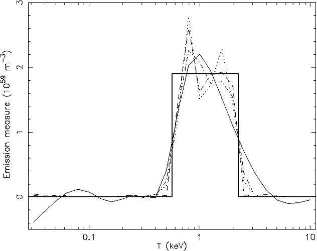 |
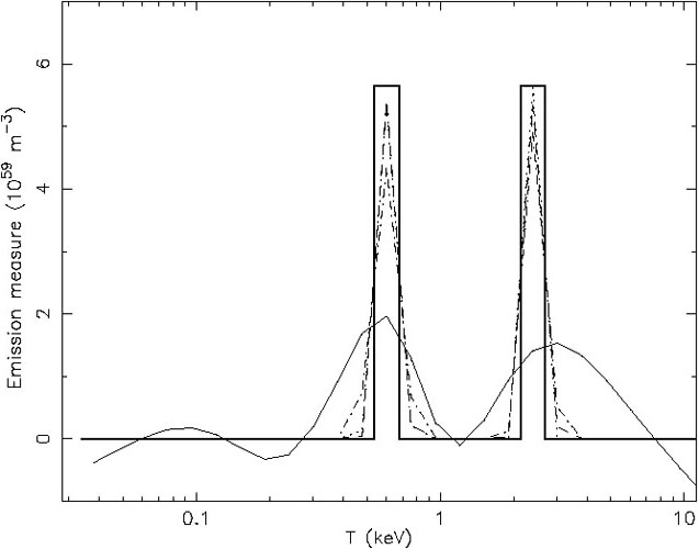
Figure 16. Reconstructed DEM
distribution for a simulated spectrum containing two equally strong
isothermal components of 0.6 and 2.4 keV (left panel) or a
uniform distribution between 0.6 and 2.4 keV (right panel). Thick solid
line: the input model; thin solid line: regularisation method;
dot-dashed line: polynomial method; dashed line: genetic algorithm;
dotted line: two broadened Gaussian components. The corresponding
best-fit spectra differ in
|
|
There are several methods to reconstruct D(T). We refer
here to
Kaastra et
al. (1996a)
for more details. All these methods have been implemented
in SPEX. They have been applied to stellar coronae or Solar spectra, but
recently also to clusters of galaxies. See for example
Kaastra (2004).
In the last case, an analytical power-law approximation D(T)
~ T 1 /
 has been used.
Also for photo-ionised plasmas a similar technique can be
applied. Instead of the temperature T, one uses the ionisation
parameter  (XSTAR
users) or U (Cloudy users). In some cases
(like Seyfert 2 galaxies with emission spectra) one recovers
D() from
the observed emission spectra; in other cases (like
Seyfert 1 galaxies with absorption spectra), a continuum model is
applied to the observed spectrum, and
D() is
recovered from
the absorption features in the spectrum. Most of what has been said
before on D(T) also applies to this case, i.e. the
resolution in
and the various methods to reconstruct the continuous
distribution D().
(XSTAR
users) or U (Cloudy users). In some cases
(like Seyfert 2 galaxies with emission spectra) one recovers
D() from
the observed emission spectra; in other cases (like
Seyfert 1 galaxies with absorption spectra), a continuum model is
applied to the observed spectrum, and
D() is
recovered from
the absorption features in the spectrum. Most of what has been said
before on D(T) also applies to this case, i.e. the
resolution in
and the various methods to reconstruct the continuous
distribution D().
The authors thank ISSI (Bern) for support of the team "Non-virialized X-ray components in clusters of galaxies". SRON is supported financially by NWO, the Netherlands Organization for Scientific Research.
1 http://www.arcetri.astro.it/science/chianti/chianti.html Back.
2 http://cxc.harvard.edu/atomdb Back.
3 http://heasarc.gsfc.nasa.gov/docs/xanadu/xspec Back.
4 http://www.sron.nl/spex Back.
5 http://heasarc.gsfc.nasa.gov/docs/software/xstar/xstar.html Back.
6 http://www.nublado.org Back.
 2
by less than 2 for each case. Obviously, small scale detail cannot be
recovered but bulk properties such as the difference between a bimodal
DEM distribution (left panel) or a flat distribution (right panel) can
be recovered. From
(
2
by less than 2 for each case. Obviously, small scale detail cannot be
recovered but bulk properties such as the difference between a bimodal
DEM distribution (left panel) or a flat distribution (right panel) can
be recovered. From
(