2. BASIC EQUATIONS FOR CHEMICAL EVOLUTION

2.1. Yields per Stellar Generation

Under the assumption of Instantaneous Recycling Approximation (IRA) which states that all stars more massive than 1 M die immediately, whereas all stars with masses lower than 1 M live forever, one can define the yield per stellar generation (Tinsley, 1980):

(20)

where p_im is the stellar new yield of the element i, namely the newly formed and ejected element i by a star of mass m, and (m) is the IMF.

The quantity R is the so-called Returned Fraction:

(21)

and is the mass fraction of gas restored into the ISM by an entire stellar generation. The term fraction derives from the fact that in its definition R is divided by ₀ m (m) dm = 1, which is the normalization condition for the IMF. Therefore, (1 - R) is the fraction of mass locked up in very low mass stars and remnants.

2.2. Analytical models

Simple Model

The Simple Model for the chemical evolution of the solar neighbourhood is the simplest approach to model chemical evolution. The solar neighbourhood is assumed to be a cylinder of 1 Kpc radius centered around the Sun.

The basic assumptions of the Simple Model are:

- the system is one-zone and closed, no inflows or outflows are considered,

- the initial gas is primordial (no metals),

- IRA holds,

- the IMF, (m), is assumed to be constant in time,

- the gas is well mixed at any time (instantaneous mixing approximation, IMA).

The Simple Model fails in describing the evolution of the Milky Way (G-dwarf metallicity distribution, elements produced on long timescales and abundance ratios) and the reason is that at least two of the above assumptions are manifestly wrong, epecially if one intends to model the evolution of the abundance of elements produced on long timescales, such as Fe. In particular, the assumptions of the closed box and the IRA.

However, it is interesting to know the solution of the Simple Model and its implications. Let Z be the abundance by mass of metals, then we obtain the analytical solution of the Simple Model by ignoring the stellar lifetimes:

(22)

where G = M_gas / M_tot is the gas mass fraction of the system and y_Z is the yield per stellar generation, as defined above, otherwise called effective yield.

In particular, the effective yield is defined as:

(23)

namely the yield that the system would have if behaving as the simple closed-box model. This means that if y_Zeff > y_Z, then the actual system has attained a higher metallicity at a given gas fraction G. Generally, given two chemical elements i and j, the solution of the Simple Model for primary elements (eq. 22) implies:

(24)

which means that the ratio of two element abundances is always equal to the ratio of their yields. This is no more true when IRA is relaxed. In fact, relaxing IRA is necessary to study in detail the evolution of the abundances of single elements produced on long timescales (e.g. Fe, N).

Analytical models in the presence of outflows

One can obtain analytical solutions also in the presence of infall and/or outflow but the necessary condition is to assume IRA, as well as precise forms for the infall and outflow rates.

Matteucci & Chiosi (1983) found solutions for models with outflow and infall and Matteucci (2001) found it for a model with infall and outflow acting at the same time. The main assumption in the model with outflow but no infall is that the outflow rate is:

(25)

where > 0 is the wind parameter.

The solution of this model is:

(26)

for = 0 the equation becomes the one of the Simple Model (eq. 22).

As one can see from eq. (26), the presence of an outflow decreases the effective yield, in the sense that the true yield of a system is lower than the effective yield. Models with galactic winds or outflows in general are suitable for ellipticals, irregulars and for the Galactic halo. A popular analytical model with outflow is that suggested by Hartwick (1976) for the evolution of the Galactic halo, under the assumption that during the halo collapse stars were forming while the gas was dissipating energy and falling into the bulge and disk, thus producing a net gas loss from the halo. This hypothesis was suggested by the fact that the stellar metallicity distribution of the halo can be reproduced only with an effective yield lower than that of the disk. In Hartwick's model the ouflow rate is assumed to be simply proportional to the SFR:

(27)

which is similar to eq. (25). Hartwick used this model to reproduce the metallicity distribution of halo stars and also to alleviate the G-dwarf problem in the disk, namely the fact that the Simple Model of chemical evolution predicts too many disk stars than observed (see Tinsley 1980 for a review on the subject). However, the gas lost from the halo cannot have contributed to form the whole disk since the distribution of the specific angular momentum of halo and disk stars are quite different, thus indicating that only a negligible amount of halo gas can have formed the disk. On the other hand, the similarity of the distributions for the halo and bulge indicates that the bulge must have formed out of gas lost from the halo (see Wyse & Gilmore 1992). The G-dwarf problem is instead easily solved if one assumes that the Galactic disk has formed by means of slow infall of extragalactic material, as we will see in the next sections. Recently, Hartwick's model has been revisited by Prantzos (2003) to interpret the most recent metallicity distribution of halo stars, which is quite different with respect to the G-dwarf metallicity distribution in the local disk. In particular, the halo metallicity distribution is peaked at around [Fe/H] = -1.6 dex, whereas the G-dwarf distribution is peaked at around ~ -0.2 dex. Prantzos (2003) suggested that an outflow with = 8 as well as a formation of the halo by early infall are necessary to reproduce the observed halo metallicity distribution. In Figure 11 we show the results of Prantzos (2003) compared with observations.

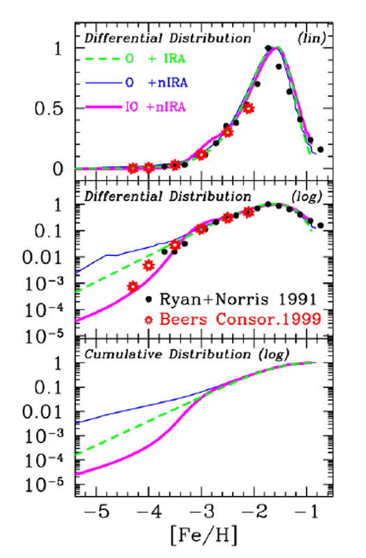Figure 11. Metallicity distribution for the halo stars. Upper panel: observed and predicted metallicity distributions. The models are: pure outflow with IRA (dashed curve), pure outflow without IRA (thin solid curve) and early infall +outflow without IRA (thick solid curve). The distribution is on a linear scale. Middle panel: the same as above but the distribution is on a logarithmic scale. Lower panel: predicted cumulative distributions. Figure from Prantzos (2003).

Analytical models in presence of infall

The solution of the equation of metals for a model without a wind but with a primordial infalling material (Z_A = 0) at a rate:

(28)

and 1 is :

(29)

For = 1 one obtains the well known case of extreme infall studied by Larson (1972) whose solution is:

(30)

This extreme infall solution shows that when G 0 then Z y_Z. The infall can solve the G-dwarf problem for disk stars except for the extreme infall solution which predicts too few low metallicity stars below [Fe/H] = -1.0 (see Tinsley 1980). Finally, we can conclude that the infall is very important for explaining both the halo and the disk formation.

Analytical models in presence of infall and outflow

Matteucci (2001) presented an analytical solution for infall and outflow present at the same time. The solution refers to the outflow and infall rates of eq. (25) and eq. (28), respectively.

In particular:

(31)

for a primordial infalling gas (Z_A = 0). This solution is velid for > 0 and > 0 and 1.

2.3. Detailed numerical models

Detailed models of galactic chemical evolution require consideration of the stellar lifetimes, namely they should relax IRA. However, the majority of them still retain the instantaneous mixing approximation (IMA), which assumes that the material ejected by stars at their death is instantaneously mixed with the surrounding interstellar medium (ISM). This approximation seems to be good in the majority of the cases with perhaps the exception of the very early phases of galactic evolution.

The basic equations of chemical evolution follow the evolution of the abundances of single chemical species and the gas as a whole.

If _i is the surface mass density of an element i, with _gas = _{i = 1,n i} being the total surface gas density and n the total number of chemical elements, we can write:

(32)

for any ggiven chemical element. These equations can be solved only numerically. The quantities X_i(t) are the abundances as defined in eq. (1). The quantity Q_mi contains all the information about stellar evolution and nucleosynthesis: in practice it gives the mass of gas produced and ejected in the form of an element i by a star of initial mass m, together with the mass of that element which was already present in the star at birth. The various integrals represent the rates at which the mass of a given element is restored into the ISM by stars of different masses which can evolve into WDs or supernovae (II, Ia, Ib). The integral representing the rate of matter restoration by Type Ia SNe is the second one on the right hand side. The quantity A is a constant: it is the fraction, in the IMF, of binary systems with those specific features required to give rise to Type Ia SNe, whereas B=1-A is the fraction of all the single stars and binary systems in the same mass range of definition of the progenitors of Type Ia SNe (third integral). The parameter A is obtained by imposing that the predicted Type Ia SN rate reproduces the observed rate at the present time (14 Gyr). Values of A = 0.05-0.09 are found for the evolution of the solar vicinity when an IMF of Scalo (1986, 1998) or Kroupa et al. (1993) is adopted. If one adopts a flatter IMF such as the Salpeter (1955) one, then A is different. The integral of the Type Ia SN contribution is made over a range of mass going from M_Bm = 3 M to M_BM = 16 M, which represents the total masses of binary systems able to produce Type Ia SNe in the framework of the single degenerate scenario. There is also an integration over the mass distribution of binary systems; in particular, one considers the function f() where = M₂ / (M₁ + M₂), with M₁ and M₂ being the primary and secondary mass of the binary system, respectively (for more details see Matteucci & Greggio 1986 and Matteucci 2001). The third and fourth integrals represent the rates of Type II and Type Ib/c SNe, respectively. The occurrence of Type Ib SNe seems to be partly related to Wolf-Rayet stars which have original masses larger tham 25 M and depends on the mass loss rate which is more active at high metallicities. However, it has been proposed that Type Ib SNe can also originate from massive stars in binary systems. Finally, the functions A(t) and W(t) are the infall and wind rate, respectively.