


A different pattern for the
[ /Fe] vs. [Fe/H]
relation compared to the solar vicinity is observed in dwarf spheroidal
galaxies (dSphs) of the Local Group, as shown in
Figure 43, and this can be easily interpreted
in the framework of the time-delay model coupled with different star
formation histories.
/Fe] vs. [Fe/H]
relation compared to the solar vicinity is observed in dwarf spheroidal
galaxies (dSphs) of the Local Group, as shown in
Figure 43, and this can be easily interpreted
in the framework of the time-delay model coupled with different star
formation histories.
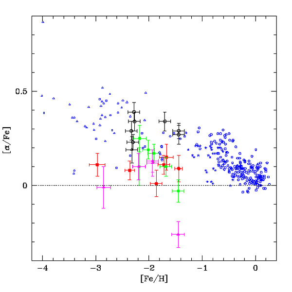 |
Figure 43. Observed
[ |
Before interpreting the
[/Fe] diagram, we recall
the current ideas about the formation of the dSphs.
Cold dark matter (CDM) models for galaxy formation predict that the
dSphs, systems with luminous masses of the order of 107
M , are
the first objects to form stars and that all stars in these systems
should form on a timescale < 1 Gyr, since the heating and gas loss,
due to reionization, must have halted the SF soon.
However, observationally all dSph satellites of the Milky Way contain
old stars indistinguishable from those of Galactic globular clusters and
they seem to have experienced SF for long periods (> 2 Gyr,
Grebel &
Gallagher 2004).
The histories of SF for these galaxies are generally derived from the
color-magnitude diagram (e. g.
Mateo 1998).
By looking at the [/Fe]
vs. [Fe/H] relations for dSphs, as shown in
Figure 43, one can immediately suggest, on the
basis of the time-delay model, that their evolution should have been
characterized by a slow and protracted SF, at variance with the
suggestion of a fast episode of SF truncated by the heating due to
reionization.
, are
the first objects to form stars and that all stars in these systems
should form on a timescale < 1 Gyr, since the heating and gas loss,
due to reionization, must have halted the SF soon.
However, observationally all dSph satellites of the Milky Way contain
old stars indistinguishable from those of Galactic globular clusters and
they seem to have experienced SF for long periods (> 2 Gyr,
Grebel &
Gallagher 2004).
The histories of SF for these galaxies are generally derived from the
color-magnitude diagram (e. g.
Mateo 1998).
By looking at the [/Fe]
vs. [Fe/H] relations for dSphs, as shown in
Figure 43, one can immediately suggest, on the
basis of the time-delay model, that their evolution should have been
characterized by a slow and protracted SF, at variance with the
suggestion of a fast episode of SF truncated by the heating due to
reionization.
The dSph satellites of the Milky Way are considered the smallest dark
matter dominated systems in the universe.
In the past years there have been a few attempts at deriving the amount
of dark matter in dSphs, in particular by measuring the mass to light
ratios versus magnitude for these galaxies (e.g.
Mateo 1998;
Gilmore et
al. 2007).
Gilmore et
al. (2007)
suggested that the dSphs have a shallow central dark matter distribution
and no galaxy is found with a dark mass halo less massive than 5 ×
107
M, as
shown in Figure 44.
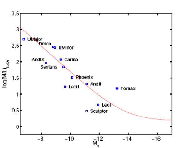 |
Figure 44. Dark matter in dSphs: mass to
light ratios versus absolute
V magnitude for some Local Group dSphs. The solid curve shows the
relation expected if all the dSphs contain about 4 ×
107
M |
In recent years there has been a fast development in the field of
chemical evolution of dSphs of the Local Group due to the increasing
amount of data on chemical abundances derived from high resolution
spectra (e.g.
Smecker-Hane &
McWilliam, 1999;
Bonifacio el al. 2000,
2004;
Shetrone et
al. 2001,
2003;
Tolstoy et
al. 2004;
Bonifacio et
al. 2004;
Venn et al. 2004;
Sadakane et
al. 2004;
Fulbright et
al. 2004;
McWilliam &
Smecker-Hane 2005a,
b;
Monaco et
al. 2005;
Geisler et
al. 2005).
The abundances of
-elements (O, Mg, Ca,
Si,) plus the abundances of s- and r- process elements (Ba, Y, Sr, La
and Eu) were measured with unprecedented accuracy. Besides these
high-resolution studies we recall also the measure of the metallicities
of many red giant stars in several dSphs by
Tolstoy et
al. (2004),
Koch et al. (2006),
Helmi et al. (2006)
and
Battaglia et
al. (2006)
obtained from the low-resolution Ca triplet. An interesting result of
Helmi et al. (2006)
is that they did not find stars with [Fe/H] < -3.0 dex and that the
metallicity distribution of the stars in dSphs is different from that of
halo stars in the Milky Way.
Other important information, as already mentioned, comes from the
photometry of dSphs of the Local Group and in particular from the
color-magnitude diagrams. From these diagrams one can infer the history
of SF of these galaxies. We recall the studies of
Hernandez et
al. (2000),
Dolphin (2002),
Bellazzini et
al. (2002),
Rizzi et al. (2003),
Monelli et
al. (2003),
Dolphin et
al. (2005).
The color-magnitude diagrams seem
to indicate that the majority of dSphs had one rather long episode of SF
with the exception of Carina for which four episodes of SF have been
suggested
(Rizzi et al. 2003).
Several papers have appeared in the last few
years concerning the chemical evolution of dSphs. For example
Carigi et
al. (2002)
computed models for the chemical evolution of
four dSphs by adopting the SF histories derived, from color-magnitude
diagrams, by
Hernandez et
al. (2000).
In their model they assumed gas infall
and computed the gas thermal energy heated by SNe in order to study
galactic winds. In fact, the dSphs must have lost their gas in one way
or another (galactic winds and/or ram pressure stripping) since they
appear completely without gas. They assumed that the wind is sudden and
devoids the galaxy of gas instantaneously. The adopted IMF is the
Kroupa et al. (1993)
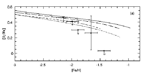
IMF as in the solar vicinity. They predicted a too high metallicity for Ursa Minor and did not match the
correct slope for the observed
[/Fe] ratios, unless the
history of SF in this galaxy was assumed to be different than suggested
by its color-magnitude diagram, as shown in
Figure 45.
 |
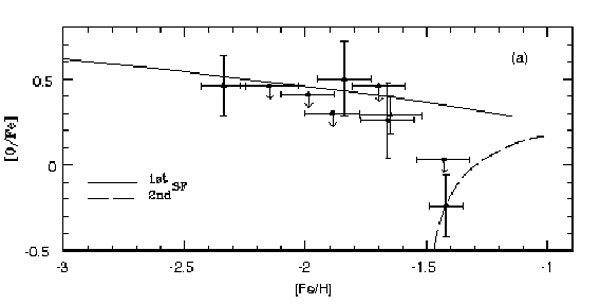 |
Figure 45. Observed and predicted [O/Fe] vs. [Fe/H] relation for the galaxy Ursa Minor. Models and Figures by Carigi et al. (2002). The upper Figure presents models assuming only one burst of SF at high redshift, as suggested by the color-magnitude diagram of this galaxy. The lower Figure shows the predictions of a model with two separate bursts which seems to fit better the data. |
Then, Ikuta & Arimoto (2002) proposed a closed box model (no infall nor outflow) for dSphs. In this Simple Model they had to assume some external cause to stop star formation, such as ram pressure stripping. They tested different IMFs and suggested that these galaxies had suffered very low SFRs (1-5% of that in the solar neighbourhood) and that the SF had a long duration (> 3.9-6.5 Gyr). In Figure 46 are shown their predictions for [Mg/Fe] in dSphs. Also here, the predicted slope of the [Mg/Fe] ratio is flatter than observed.
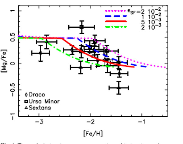 |
Figure 46. Observed and predicted [Mg/Fe]
vs. [Fe/H] relation for the dSph Draco, Ursa Minor and Sextans. The
different curves refer to different SF efficiencies
( |
More recently, Fenner et al. (2006) suggested a model with a galactic wind for Sculptor: they indicated an efficiency of SF of 0.05 Gyr-1. They concluded, from the study of the [Ba/Y] ratio, that chemical evolution in dSphs is inconsistent with the SF being truncated after reionization (at redshift z = 8). In fact, the high value of this ratio measured in stars indicates strong s-process production from low mass stars which have very long lifetimes.
The results of Lanfranchi & Matteucci
Lanfranchi & Matteucci (2003; 2004 hereafter LM04) developed models for dSphs of the Local Group. First they tested a "standard model" devised for describing an average dSph galaxy. This model was based on the following assumptions:
 (wind parameter)
between 5 and 15.
(wind parameter)
between 5 and 15.
The condition for the onset of the wind is written as:
 |
(37) |
namely, that the thermal energy of the gas is larger or equal to its binding energy. The thermal energy of gas due to SN and stellar wind heating is:
 |
(38) |
with the contribution of SNe being:
 |
(39) |
while the contribution of stellar winds is:
 |
(40) |
with
 SN =
SN =
 SN
o and
o =
1051 erg (typical SN energy), and
w =
w
Ew with Ew = 1049 erg
(typical energy injected by the stellar wind of a 20
M star
taken as representative).
w
and
SN
are two free parameters and indicate the efficiency of
energy transfer from stellar winds and SNe into the ISM, respectively,
quantities still largely unknown. It is assumed that
w = 0.03
for the stellar winds, and that
SN = 0.03
for Type II SNe and
SN = 1.0
for Type Ia SNe, as suggested by
Recchi et
al. (2001).
The total mass of the galaxy is expressed as
Mtot(t) =
M*(t)
+ Mgas(t) + Mdark(t)
with ML(t) =
M*(t) + Mgas(t)
and the binding energy of gas is:
SN
o and
o =
1051 erg (typical SN energy), and
w =
w
Ew with Ew = 1049 erg
(typical energy injected by the stellar wind of a 20
M star
taken as representative).
w
and
SN
are two free parameters and indicate the efficiency of
energy transfer from stellar winds and SNe into the ISM, respectively,
quantities still largely unknown. It is assumed that
w = 0.03
for the stellar winds, and that
SN = 0.03
for Type II SNe and
SN = 1.0
for Type Ia SNe, as suggested by
Recchi et
al. (2001).
The total mass of the galaxy is expressed as
Mtot(t) =
M*(t)
+ Mgas(t) + Mdark(t)
with ML(t) =
M*(t) + Mgas(t)
and the binding energy of gas is:
 |
(41) |
with:
 |
(42) |
which is the potential well due to the luminous matter and with:
 |
(43) |
which represents the potential well due to the interaction between dark and
luminous matter, where wLD ~ (1 /
2 ) S(1 + 1.37S),
with S = rL / rD, being the
ratio between the galaxy effective radius and the radius of the dark
matter core. The typical model for a dSph starts with an initial
baryonic mass of 108
M and
ends up, after the wind, with a luminous mass of ~ 107
M.
The dark matter halo is assumed to be ten times larger than the luminous
mass but diffuse (S = 0.1). The galactic wind in these galaxies
develops after several Gyr from the start of SF, according to the
different assumed SF efficiency. Soon after, but not immediately, the
wind has started, the SF decreases very strongly until it halts completely.
) S(1 + 1.37S),
with S = rL / rD, being the
ratio between the galaxy effective radius and the radius of the dark
matter core. The typical model for a dSph starts with an initial
baryonic mass of 108
M and
ends up, after the wind, with a luminous mass of ~ 107
M.
The dark matter halo is assumed to be ten times larger than the luminous
mass but diffuse (S = 0.1). The galactic wind in these galaxies
develops after several Gyr from the start of SF, according to the
different assumed SF efficiency. Soon after, but not immediately, the
wind has started, the SF decreases very strongly until it halts completely.
In Figure 47 we show the
[/Fe] ratios for different
-elements and for
different efficiencies of SF, as predicted by the standard model of
Lanfranchi &
Matteucci (2003).
 |
Figure 47. Observed and predicted
[ |
As one can see, the
[/Fe] ratios show a
clear change in slope followed by a steep decline, in agreement with the
data. The change in slope corresponds to the occurrence of the galactic
wind which starts emptying the galaxy of gas. In such a situation the SF
starts to decrease as does therefore the production of the
-elements from massive
stars, whereas Fe continues to be produced since its progenitors have
long lifetimes. This produces the steep slope: the low SF efficiency and
the wind, which decreases furtherly the SF. In this situation, the
time-delay model predicts an earlier and steeper decline of the
[/Fe] ratios, as we have
already discussed.
In LM04, the histories of star formation of specific galaxie, as suggested by their color-magnitude diagrams, were taken into account, and they developed models for six dSphs: Carina, Ursa Minor, Sculptor, Draco, Sextans and Sagittarius. In Table 1 we show the assumed SF formation histories and model parameters. In particular, in column 1 are the galaxy names, in column 2 are the initial baryonic masses, in column 3 are the SF efficiencies, in column 4 are the wind parameters, in column 5 are the numbers of SF episodes, in column 6 are the times at which the SF episodes start, in column 7 are the durations, in Gyr, of the SF episodes and in column 8 the assumed IMF.
| galaxy | Mtotinitial
(M) |
 (Gyr-1) (Gyr-1) |
|
n | t(Gyr) | d(Gyr) | IMF |
| Sextan | 5 * 108 | 0.01-0.3 | 9-13 | 1 | 0 | 8 | Salpeter |
| Sculptor | 5 * 108 | 0.05-0.5 | 11-15 | 1 | 0 | 7 | Salpeter |
| Sagittarius | 5 * 108 | 1.0-5.0 | 9-13 | 1 | 0 | 13 | Salpeter |
| Draco | 5 * 108 | 0.005-0.1 | 6-10 | 1 | 6 | 4 | Salpeter |
| Ursa Minor | 5 * 108 | 0.05-0.5 | 8-12 | 1 | 0 | 3 | Salpeter |
| Carina | 5 * 108 | 0.02-0.4 | 7-11 | 2 | 6/10 | 3/3 | Salpeter |
In Figures 48, 49,
50, 51 and
52 we show the predictions for specific dSphs
by LM04. As one can see, the
[/Fe] data in the dSphs
are well reproduced and in particular the steep decline of the
[/Fe] ratio is well
reproduced. This steep decline is due again to the low efficiency SFR, a
feature common also to the other
models, coupled with a strong and continuous galactic wind which
gradually empties the galaxies of gas. In the previous models either the
galactic wind was not present or it was assumed instantaneous or not as
strong as in LM04, thus predicting a flatter slope for the descent of
the [/Fe] vs. [Fe/H], as
we have already seen.
 |
Figure 48. Observed and predicted
[ |
 |
Figure 49. Observed and predicted
[ |
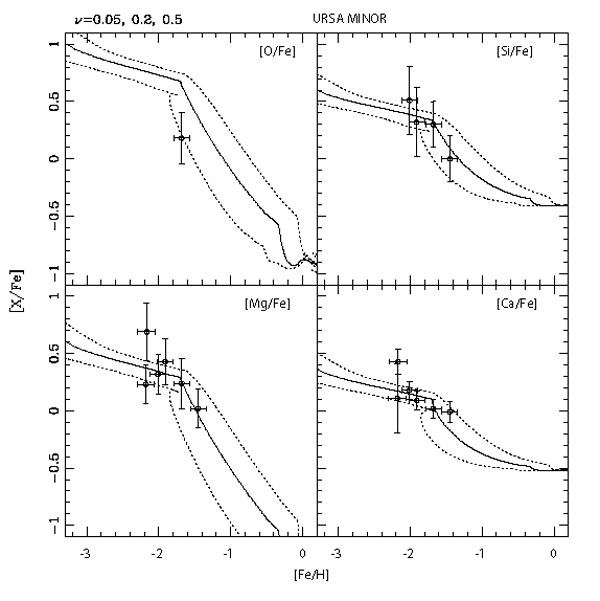 |
Figure 50. Observed and predicted
[ |
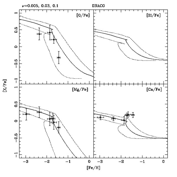 |
Figure 51. Observed and predicted
[ |
 |
Figure 52. Observed and predicted
[ |
Lanfranchi et
al. (2006)
computed also the expected abundances of s- and r- process elements in
dSphs, by adopting the same nucleosynthesis prescriptions used for the
chemical evolution of the Milky Way. In particular, they adopted the
prescriptions of
Cescutti et
al. (2006)
for Ba, Y, La, Sr and Eu: Ba, Sr , La and Y are mainly s-process
elements produced on long timescales by low mass stars (1-3
M), but
they have also a small r-process component originating in stars in the
mass range 12-30
M. The
Eu instead is considered as a pure r-process element produced in the
stellar mass range 12-30
M.
In Figures 53, 54,
55 and 56 we show the
predictions of
Lanfranchi et
al. (2006)
for s-and r-process elements in dSphs compared with the available
data. Also in this case the agreement looks good, although more data are
necessary before drawing firm conclusions. The general tendency for the
-elements in dSphs is to
be less overabundant relative to Fe and the Sun than the stars of the
solar vicinity with the same [Fe/H]. This is due to the lower SFR in
dSphs (the effect is increased by the galactic
wind) which acts to shift the curve
[/Fe] vs. [Fe/H] for the
solar vicinity towards left in the diagram, whereas a stronger SF than
in the solar neighbourhood moves the solar vicinity curve toward right
in the diagram (see Figure 33).
The same holds for s- and r- process elements: in this case, since
[s/Fe] vs. [Fe/H] first increases sharply at low metallicities and then
it flattens at higher ones (the opposite of what happens for the
-elements), the dSphs
show a higher [s/Fe] than the stars in the solar vicinity at the same
[Fe/H]. This shows again the effect of the time-delay model.
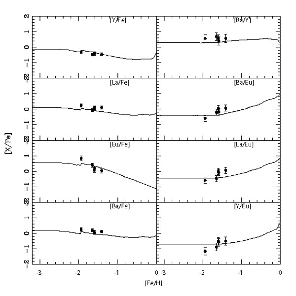 |
Figure 53. Predicted and observed [s,r/Fe] vs. [Fe/H] for the galaxy Carina. The model is from Lanfranchi, Matteucci & Cescutti (2006a), where the references for the data can be found. |
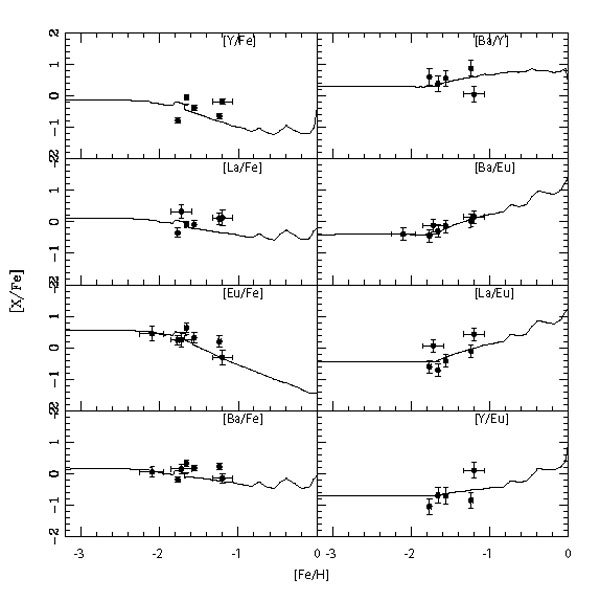 |
Figure 54. Predicted and observed [s,r/Fe] vs. [Fe/H] for the galaxy Sculptor. The model is from Lanfranchi, Matteucci & Cescutti (2006a), where the references for the the data can be found. |
 |
Figure 55. Predicted and observed [Ba/Eu] vs. [Fe/H] for the galaxy Sculptor. The model is from Lanfranchi, Matteucci & Cescutti (2006a), the data and the figure are from Geisler et al. (2007). |
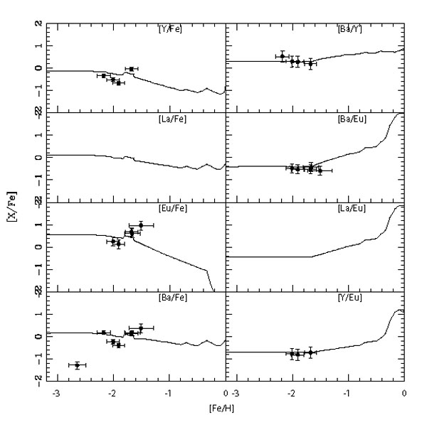 |
Figure 56. Predicted and observed [s,r/Fe] vs. [Fe/H] for the galaxy Ursa Minor. The model is from Lanfranchi, Matteucci & Cescutti (2006a), where the references for the the data can be found. |
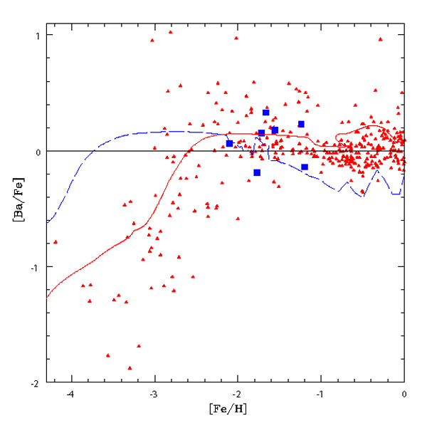
The differences between the [s/Fe] vs. [Fe/H] in dSphs and the Milky Way are shown in Figures 57, where data and predictions of Ba and Eu for Sculptor are compared with data and predictions of Ba and Eu in the solar vicinity.
 |
 |
Figure 57. Comparison between data and predictions for Ba and Eu in Sculptor and in the Milky Way. Model for the Milky Way: continuous lines. Model for Sculptor: dashed lines. Data for the Milky Way: triangles. Data for Sculptor: full squares. Models from Lanfranchi & al. (2007) where the references to the data can be found. |
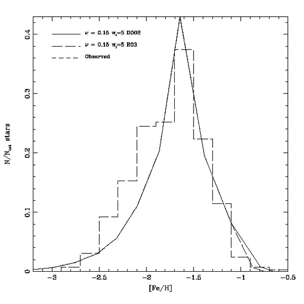
Finally, another important constraint for models of galactic chemical evolution is represented by the stellar metallicity distribution. In Figures 58 we show the predictions for the stellar metallicity distribution of Carina compared with the observed one and the agreement is very good. The observed distribution is from Koch et al. (2006) who measured the metallicity of 437 giants in Carina by means of Ca triplet and then transformed it into [Fe/H] through a suitable calibration. In Figures 58 we also show the comparison between the stellar metallicity distribution in Carina and the G-dwarf metallicity distribution in the solar vicinity. As one can see, the Carina distribution lies in a range of smaller metallicities due to the lower efficiency of SF assumed for this galaxy.
 |
 |
Figure 58. Upper panel: stellar metallicity
distribution for Carina. Model from
Lanfranchi et
al. (2006b).
The assumed SF efficiency is |
To this purpose, owing a word of caution is appropriate: in fact, the Ca triplet in principle traces the abundance of Ca and not that of Fe and we know that Ca and Fe evolve in a different way since Ca is mainly produced in Type II SNe, whereas Fe is produced mainly in Type Ia SNe. This different evolution of Ca and Fe leads, in the Koch paper, to an uncertainty of 0.2 dex. Besides that, the globular clusters which serve as calibrators for obtaining [Fe/H] lie in the range -2.0 - -1.0 dex, whereas Koch's data extend down to lower metallicities.
The good fit of the stellar metallicity distribution indicates that both the assumed history of SF and the IMF are close to reality.
LM04 predicted the stellar metallicity distribution for all the six dSphs and while for Carina the agreement is quite good for Sculptor they cannot reproduce the bimodal stellar distribution recently suggested by Tolstoy et al. (2004) and shown in Figure 59, since their model is a one-zone model. In Figure 60 are shown the predictions of LM04 for the Sculptor galaxy: it is clear from this Figure that to reproduce the two different stellar populations, one has to assume a multizone model possibly with different efficiencies of SF. Kawata et al. (2006) explained the bimodality of stellar populations in Sculptor as a consequence of dissipative collapse which produces higher metallicities at the center of the galaxy.
 |
Figure 59. Observed stellar metallicity distribution for Sculptor. Data and figure are from Tolstoy et al. (2004): all the stars of Sculptor are indicated by the dotted line. The central stars are those indicated by the lower histogram with continuous line, whereas the stars beyond R > 0.2 Kpc are indicated by the upper histogram with continuous line. |
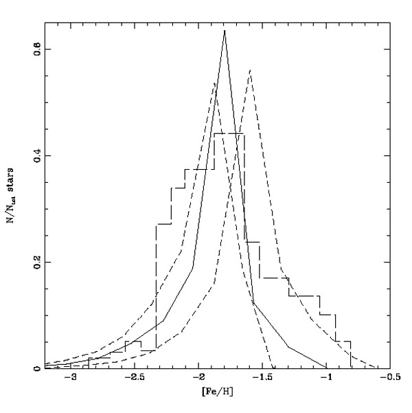 |
Figure 60. Observed and predicted stellar metallicity distribution for Sculptor. The data (the dotted line of Figure 59) are represented by the histogram (long dashed). The models are from LM04: the solid line represents the best model, whereas the dashed lines represent models with higher (the curve on the right) or lower (the curve on the left) SF efficiency. |