


With the name cosmic chemical evolution we indicate the chemical
evolution taking place in comoving volumes large enough to be
representative of the whole universe
(Pei & Fall
1995).
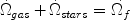
The evolution can be described in terms of comoving densities of gas and
stars  gas
and
stars,
both measured in units of the present critical density
(
gas
and
stars,
both measured in units of the present critical density
( c =
3Ho2 /
(8
c =
3Ho2 /
(8  G)) and the mean
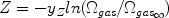
abundance of heavy elements in the ISM, Z, including dust.
Under IRA we can write, following Pei & Fall:
G)) and the mean
abundance of heavy elements in the ISM, Z, including dust.
Under IRA we can write, following Pei & Fall:
 |
(44) |
and
 |
(45) |
where the dots represent differentiation with respect to the cosmic time.
The term f
can represent either the infall or the outflow rate according to its sign.
For the closed-box model
f = 0 and
its solution is:
 |
(46) |
with gas being the gas comoving density at some suitably
high redshift when there are still no stars and heavy elements.
being the gas comoving density at some suitably
high redshift when there are still no stars and heavy elements.
By means of these equations Pei & Fall followed the evolution of DLAs
(the quasar absorbers). They expressed the quantity
gas in
terms of the observable properties of DLAs. They assumed IRA.
Since all these cosmic quantities refer to an unitary volume of the universe which contains galaxies of all morphological types,
Calura & Matteucci (2004) proposed another approach to the cosmic chemical evolution, which takes into account galaxies of different morphological type. They computed the cosmic chemical enrichment of the universe by means of detailed models of chemical evolution of galaxies of all morphological types, relaxing IRA and assuming for each galaxy type a different history of SF, as discussed in the previous sections. They defined the comoving cosmic density of stars and gas for galaxies of different morphological type (ellipticals, spirals and irregulars) as:
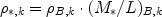 |
(47) |
for the stars and
 |
(48) |
for the gas. The quantities (M* /
L)B,k and (Mg /
L)B,k are the
predicted M/L ratios for stars and gas, respectively.
LB,k is the blue luminosity for each galaxy type
(k indicates the morphological type) and
B,k
is the comoving luminosity for a given galaxian morphological type.
They computed the mean mass weighted metallicity of galaxies by summing the metallicities predicted for the different morphological types as:
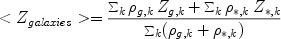 |
(49) |
and obtained:
 |
(50) |
where Z = 0.02 and with 56%, 42% and 2% of metals produced in ellipticals,
spirals and irregulars, respectively. Therefore, the conclusion is that
the average metallicity in galaxies is almost solar and that most of the
metals in the universe have been produced by elliptical galaxies. They
also predicted the average [O/Fe] ratios for each galaxy type both in
the gas and in stars.
= 0.02 and with 56%, 42% and 2% of metals produced in ellipticals,
spirals and irregulars, respectively. Therefore, the conclusion is that
the average metallicity in galaxies is almost solar and that most of the
metals in the universe have been produced by elliptical galaxies. They
also predicted the average [O/Fe] ratios for each galaxy type both in
the gas and in stars.
In particular:
[O/Fe]*,Ellipt = 0.4 dex, [O/Fe]gas,Ellip = -0.33 dex, [O/Fe]*,Spiral = 0.1 dex and [O/Fe]gas,Spiral = 0.01 dex.
Then, they computed the metallicity in the intergalactic medium (IGM) by considering all the metals ejected by galaxies (mainly ellipticals) into the IGM:
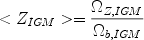 |
(51) |
with b,IGM
= b -
b,*
- b,gas =
0.0753 being the baryonic density of the IGM and
b = 0.02
h-2 (from WMAP,
Spergel et al. 2003,
2007)
being the total baryonic content of the universe. Therefore, they obtained:
 |
(52) |
Finally, they computed the average metallicity of the universe by accounting for all the metals produced in galaxies over the lifetime of the universe:
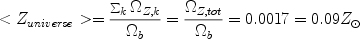 |
(53) |
where Z,tot
represents the sum of all the metals produced in all galaxies and
b
represents the the total amount of baryons in the universe.
In summary, the mean metallicity inside galaxies of all morphological types is almost solar, whereas the mean metallicity of the universe is roughly 1/10 solar.
Calura &
Matteucci (2003)
computed also cosmic Type Ia SN rates (SNRcosm),
expressed in SNu (number of SNe / 1010
LB per century). In particular, they took into
account the contribution of all galaxy types in the following way:
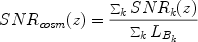 |
(54) |
where SNRcosm can represent the Type II, Ib/c, Ia SNe. The sums are over all the galactic morphological types, LBk is the total blue luminosity of the kth morphological type. In order to compute the SNRcosm for each galaxy they assumed a SN model progenitor and a cosmic SFR, calculated as:
 |
(55) |
where B,k(z) and
(M* /
L)B,k(z) have been already defined and
 (z)k represents the history of SF of a
galaxy of kth morphological type. They assumed the SF histories of
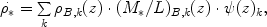
Figure 41.
In Figures 64 and 65
we show some examples of predicted cosmic SN rates by adopting the same
cosmic SFR (eq. 55) but different assumptions about the Type Ia
progenitor model.
(z)k represents the history of SF of a
galaxy of kth morphological type. They assumed the SF histories of
Figure 41.
In Figures 64 and 65
we show some examples of predicted cosmic SN rates by adopting the same
cosmic SFR (eq. 55) but different assumptions about the Type Ia
progenitor model.
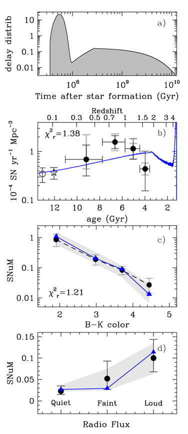 |
Figure 64. Theoretical cosmic Type Ia SN rates compared with observational data from Mannucci et al. (2006). The progenitor model adopted assumes the delay-time distribution suggested by Mannucci et al. (2005, 2006) (panel a), whereas the cosmic SFR is the one of Calura & Matteucci (2003) (panel b). In panels c) an d) are shown predictions and data for the Type Ia SN rate per unit galactic mass (SNuM) versus color and radio flux in radio galaxies, respectively. For the references about the data see Mannucci et al. (2006). Figure adapted from Mannucci et al. (2006). |
 |
Figure 65. Theoretical cosmic Type Ia SN rates compared with observational data from Mannucci et al. (2005, 2006). The progenitor model adopted assumes the delay-time distribution suggested by Matteucci & Recchi (2001) (panel a), whereas the cosmic SFR is the one of Calura & Matteucci (2003) (panel b). In panels c) an d) are shown predictions and data for the Type Ia SN rate per unit galactic mass (SNuM) versus color and radio flux in radio galaxies, respectively. For the references about the data see Mannucci et al. (2006). Figure adapted from Mannucci et al. (2006). |
As one can see from these Figures, the best DTD appears to be the one of Mannucci et al. (2006), although this conclusion is based only on the fit of the rates in radio galaxies. Concerning the cosmic Type Ia SN rate (panel b) the agreement is good for both DTDs except for the point at the highest redshift which is highly uncertain. We need more detections of SNe Ia at high redshift before drawing any conclusion on the high redshift cosmic Type Ia SN rate. In conclusion, the study of the Type Ia SN cosmic rates is very important to impose constraints on the SN progenitor model, the histories of SF in galaxies and, last but not least, the Hubble diagram.
Acknowledgement. I warmly thank Eva Grebel and Ben Moore for inviting me to deliver these lectures in the beautiful village of Murren. I also thank my collaborators, Silvia Kuna Ballero, Francesco Calura, Gabriele Cescutti, Cristina Chiappini, Gustavo Lanfranchi, Antonio Pipino and Simone Recchi, whose precious help has allowed me to put together most of the material presented in these lectures.Finally, I am grateful to I.J. Danziger for his patience in reading the manuscript.