


Modern galaxy formation theory is set within the larger scale cold dark matter cosmological model (Blumenthal et al. 1984). The success of that model in explaining the cosmic microwave background (CMB) (Komatsu et al. 2009) and large scale structure (Seljak et al. 2005, Percival et al. 2007a, Ferramacho et al. 2008, Sanchez et al. 2009) of the Universe makes it the de facto standard. However, it is important to recognize that the scales on which the simplest cold dark matter (CDM) model has been most precisely tested are much larger than those that matter for galaxy formation 1. As such, we cannot fully rule out that dark matter is warm or self-interacting, although good constraints exist on both of these properties (Markevitch et al. 2004, Boehm and Schaeffer 2005, Ahn and Shapiro 2005, Miranda and Macciò 2007, Randall et al. 2008, Yüksel et al. 2008, Boyarsky et al. 2008).
More extensive reviews of the cold dark matter cosmological model can be found in, for example, Narlikar and Padmanabhan (2001), Frenk (2002) and Bertone et al. (2005).
A combination of experimental measures, including studies of the CMB
(Dunkley et al. 2009),
large scale structure
(Tegmark et al. 2004;
Cole et
al. 2005;
Tegmark et al. 2006;
Percival
et al. 2007a,
b),
the Type Ia supernovae magnitude-redshift relation
(Kowalski et al. 2008)
and galaxy clusters
(Mantz et
al. 2009,
Vikhlinin et al. 2009,
Rozo
et al. 2010),
have now placed strong constraints on the parameters of the cold dark
matter cosmogony. The picture that emerges
(Komatsu et al. 2010)
is one in which the energy density of the Universe is shared between
dark energy
(
 =
0.728-0.016+0.015), dark matter
(c =
0.227 ± 0.014) and baryonic matter
(b =
0.0456 ± 0.0016), with a Hubble parameter
of 70.4-1.4+1.3 km/s/Mpc. Perturbations on the
uniform model seem to be well described by a scale-free primordial power
spectrum with power-law index ns = 0.963 ± 0.012
and amplitude
=
0.728-0.016+0.015), dark matter
(c =
0.227 ± 0.014) and baryonic matter
(b =
0.0456 ± 0.0016), with a Hubble parameter
of 70.4-1.4+1.3 km/s/Mpc. Perturbations on the
uniform model seem to be well described by a scale-free primordial power
spectrum with power-law index ns = 0.963 ± 0.012
and amplitude
 8 = 0.809
± 0.024.
8 = 0.809
± 0.024.
Given such a cosmological model, the Universe is 13.75 ± 0.11 Gyr old. Galaxies probably began forming at z ~ 20-50 when the first sufficiently deep dark matter potential wells formed to allow gas to cool and condense to form galaxies (Tegmark et al. 1997; Gao et al. 2007).
The formation of structure in the Universe is seeded by minute perturbations in matter density expanded to cosmological scales by inflation. The dark matter component, having no pressure, must undergo gravitational collapse and, as such, these perturbations will grow. The linear theory of cosmological perturbations is well understood and provides an accurate description of the early evolution of these perturbations. Once the perturbations become nonlinear, their evolution is significantly more complicated, but simple arguments (e.g. spherical top-hat collapse and developments thereof; Gunn 1977, Shaw and Mota 2008) provide insight into the basic behavior. Empirical methods to determine the statistical distribution of matter in the nonlinear regime exist (Hamilton et al. 1991; Peacock and Dodds 1996; Smith et al. 2003; Heitmann et al. 2009). These, together with N-body simulations (e.g. Klypin and Shandarin 1983, Springel et al. 2005b, Heitmann et al. 2008) show that a network of halos strung along walls and filaments forms, creating a cosmic web. This web is consistent with measurements of galaxy and quasar clustering on a wide range of scales.
The final result of the nonlinear evolution of a dark matter density perturbation is the formation of a dark matter halo: an approximately stable, near-equilibrium state supported against its own self-gravity by the random motions of its constituent particles. In a hierarchical universe the first halos to form will do so from fluctuations on the smallest scales. Later generations of halos can be thought of as forming from the merging of these earlier generations of halos. For the purposes of galaxy formation, two fundamental properties of the dark matter halos are of primary concern: (i) the distribution of their masses at any given redshift and (ii) the distribution of their formation histories (i.e. the statistical properties of the halos from which they formed).
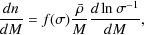
The insight of
Press
and Schechter (1974)
was that halos could be associated with peaks in the Gaussian random
density field of dark matter in the early universe. Using the relatively
simple statistics of Gaussian random fields they were able to derive the
following form for the distribution of dark matter halo masses such that
the number of halos per unit volume in the mass range M to
M +  M is
M
(dn / dM) where
2:
M is
M
(dn / dM) where
2:
 |
(1) |
where
 0
is the mean density of the Universe,
(M) is the
fractional root variance in the density field
smoothed using a top-hat filter that contains, on average, a mass
M, and
c(t)
is the critical overdensity for spherical top-hat collapse at time t
(Eke et
al. 1996).
0
is the mean density of the Universe,
(M) is the
fractional root variance in the density field
smoothed using a top-hat filter that contains, on average, a mass
M, and
c(t)
is the critical overdensity for spherical top-hat collapse at time t
(Eke et
al. 1996).
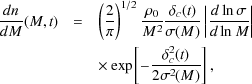
While the Press and Schechter (1974) expression is remarkably accurate given its simplicity, it does not provide a sufficiently accurate description of modern N-body measures of the halo mass function. Several attempts have been made to "fix" the Press and Schechter (1974) theory by appealing to different filters and barriers (e.g. Sheth et al. 2001) although to date none are able to accurately predict the measured form without adjusting tunable parameters. The most accurate fitting formulae currently available are those of Tinker et al. (2008; see also Reed et al. 2007, Robertson et al. 2009). Specifically, the mass function is given by
 |
(2) |
where
 |
(3) |
and where A, a, b and c are parameters
determined by fitting to the results of N-body simulations. The mass
variance
2(M)
is determined from the power spectrum of density fluctuations
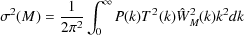 |
(4) |
where P(k) is the primordial power spectrum
(usually taken to be a scale-free power spectrum with index
ns), T(k) is the cold dark matter
transfer function
(Eisenstein and Hu 1999)
and
 M(k)
is the Fourier transform of the real-space top-hat window function.
Tinker
et al. (2008)
give values for these parameters as a function of the overdensity,
M(k)
is the Fourier transform of the real-space top-hat window function.
Tinker
et al. (2008)
give values for these parameters as a function of the overdensity,
 , used to define
what we consider to be a halo. Additionally,
they find that the best fit values are functions of redshift. Earlier
studies had hoped to find a "universal" form for the mass function (such
that the functional form was always the same when expressed in terms of
, used to define
what we consider to be a halo. Additionally,
they find that the best fit values are functions of redshift. Earlier
studies had hoped to find a "universal" form for the mass function (such
that the functional form was always the same when expressed in terms of
 =
/
c).
While this is approximately true, the work of
Tinker
et al. (2008)
demonstrates that universality does not hold when high precision results
are considered.
=
/
c).
While this is approximately true, the work of
Tinker
et al. (2008)
demonstrates that universality does not hold when high precision results
are considered.
2.3.2. Halo Formation Distribution
A statistical description of the formation of halos, specifically the sequence of merging events and the masses of halos involved in those events, can be extracted using similar arguments as the original Press and Schechter (1974) approach (Lacey and Cole 1993). These show that the distribution of halo progenitor masses, M1m at redshift z1 for a halo of mass M2 at later redshift z2 is given by
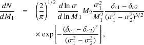 |
(5) |
where 1 =
(M1),
2 =
(M2),
c
1 = c(z1),
c
2 = c(z2). With a zero time-lag
(i.e. as z1 → z2 and therefore
c 1
→
c 2) this can be
interpreted as a merging rate (although see
Neistein
and Dekel 2008
for a counter argument). Repeated application of this merging rate can
be used to build a merger tree. Finding a suitable algorithm is
non-trivial and many attempts have been made
(Kauffmann and White 1993;
Somerville and Primack 1999;
Cole
et al. 2000;
Parkinson et al. 2008).
A recent examination of alternative algorithms is given by
Zhang et
al. (2008).
Current implementations of merger tree algorithms are highly accurate
and can reproduce the progenitor halo mass distribution over large spans
of redshift
(Parkinson et al. 2008).
A fundamental limitation of any Press and Schechter (1974) based approach is that the merger rates are not symmetric, in the sense that switching the masses M1 and M2 results in two different predictions for the rate of mergers between halos of mass M1 and M2. Benson et al. (2005) and Benson (2008) showed that a symmetrized form of the Parkinson et al. (2008) merger rate function could be made to approximately solve Smoluchowski's coagulation equation (Smoluchowksi 1916) and thereby provide a solution free from ambiguities. Other empirical determinations of merger rates have been made (Cole et al. 2008; Fakhouri and Ma 2008a, b).
In addition to these purely analytic approaches, numerical studies utilizing N-body simulations have lead to the development of an empirical understanding of halo formation histories (Wechsler et al. 2002, van den Bosch 2002) and halo-halo merger rates (Fakhouri and Ma 2008a, 2009, Stewart et al. 2009, Fakhouri et al. 2010, Hopkins et al. 2010). Merger trees can also be extracted directly from N-body simulations (e.g. Helly et al. 2003a, Springel et al. 2005b) which sidesteps these problems but incorporates any limitations of the simulation (spatial, mass and time resolution), and additionally provides information on the spatial distribution of halos. Such N-body merger trees also serve to highlight some, perhaps fundamental, limitations of the Press and Schechter (1974) type approach. For example, halos in N-body simulations undergo periods of mass loss, which is not expected in pure coagulation scenarios. The existence of systems of substructures within halos (see Section 4.1) can even lead to three-body encounters which cause subhalos to be ejected (Sales et al. 2007).
Dark matter halos are characterized by their large overdensity with
respect to the background density. Spherical top-hat collapse models
(e.g.
Eke et
al. 1996)
show that the overdensity,
, of a just
collapsed halo is
approximately 200, with some dependence on cosmological parameters. This
overdensity corresponds, approximately, to the virialized region of a
halo, and allows us to define a virial radius as
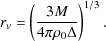 |
(6) |
Studies utilizing N-body simulations show that halos approximately obey the virial theorem within this radius and that rv is a characteristic radius for the transition from ordered inflow of matter (on larger scales) to virialized random motions (on smaller scales) (Cole and Lacey 1996). Dark matter halos have triaxial shapes and the distribution of axial ratios has been well characterized from N-body simulations (Frenk et al. 1988; Jing and Suto 2002; Bett et al. 2007).
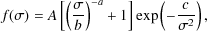
Recent N-body studies (Navarro et al. 2004; Merritt et al. 2005; Prada et al. 2006Einasto 1965) than the Navarro-Frenk-White (NFW) profile (Navarro et al. 1996, 1997). The Einasto density profile is given by
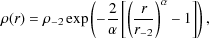 |
(7) |
where r-2 is a characteristic radius at which the
logarithmic slope of the density profile equals -2 and
 is a
parameter which controls how rapidly the logarithmic slope varies with
radius. The parameter
seems to correlate well with the height of
the peak from which a halo formed,
=
c(z)
/ (M) as has been
shown by
Gao et
al. (2008)
who provide a fitting formula,
is a
parameter which controls how rapidly the logarithmic slope varies with
radius. The parameter
seems to correlate well with the height of
the peak from which a halo formed,
=
c(z)
/ (M) as has been
shown by
Gao et
al. (2008)
who provide a fitting formula,
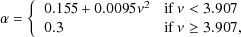 |
(8) |
which is a good match to halos in the Millennium Simulation
3
(Springel et al. 2005b).
The value of r-2 for each halo is determined from the
known virial radius, rv, and the concentration,
c-2  rv /
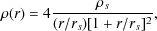
r-2. The NFW profile has a significantly simpler form
and is good to within 10-20% making it still useful. It is given by
rv /
r-2. The NFW profile has a significantly simpler form
and is good to within 10-20% making it still useful. It is given by
 |
(9) |
where rs is a characteristic scale radius and
s
is the density at r = rs. For
NFW halos, the concentration is defined as cNFW =
rv / rs.
Concentrations are found to depend weakly on halo mass and on redshift and can be predicted from the formation history of a halo (Wechsler et al. 2002). Simple algorithms to approximately determine concentrations have been proposed by Navarro et al. (1997), Eke et al. (2001) and Bullock et al. (2001b). More accurate power-law fits have also been determined from N-body simulations (Gao et al. 2008; Zhao et al. 2009).
Integrals over the density and mass distribution are needed to compute the enclosed mass, velocity dispersion, gravitational energy and so on for the halo density profile. For NFW halos the integrals are mostly straightforward, although some require numerical calculation. For the Einasto profile some of these may be expressed analytically in terms of incomplete gamma functions (Cardone et al. 2005). Specifically, expressions for the mass and gravitational potential are provided by Cardone et al. (2005), other integrals (e.g. gravitational energy) must be computed numerically.
1 Although measurements of the
Lyman- forest
(Slosar et al. 2007,
Viel et
al. 2008)
and weak-lensing
(Mandelbaum et al. 2006)
give interesting constraints on the distribution of dark matter on small
scales they typically require modeling of either the nonlinear evolution
of dark matter or the behavior of baryons (or both) which complicate any
interpretation. They are therefore not as "clean" as CMB and large scale
structure constraints.
Back.
2 The original derivation by Press and Schechter (1974) differed by a factor of 2, resulting in only half of the mass of the Universe being locked up in halos. Later derivations placed the method on a firmer mathematical basis and resolved this problem, a symptom of the "cloud-in-cloud" problem (Bond et al. 1991; Bower 1991; Lacey and Cole 1993). Back.
3 We have truncated this fit so that
never exceeds 0.3.
Gao et
al. (2008)
were not able to probe the behavior of
in the very high
regime. Extrapolating their
formula to > 4 is not
justified and we instead choose to truncate it at a maximum of
= 0.3.
Back.