1.2. CALIBRATION OF STAR FORMATION RATE INDICATORS ACROSS THE WAVELENGTH SPECTRUM

Calibrations of SFR indicators have been presented in the literature for almost 30 years, derived across the full electromagnetic spectrum, from the X-ray, through the ultraviolet (UV), via the optical and infrared (IR), all the way to the radio, and using both continuum and line emission (see review by Kennicutt 1998, and, e.g., Donas & Deharveng 1984; Yun et al. 2001; Kewley et al. 2002, 2004; Ranalli et al. 2003; Bell 2003; Calzetti et al. 2005, 2007, 2010; Schmitt et al. 2006; Alonso-Herrero et al. 2006; Moustakas et al. 2006; Salim et al. 2007; Persic & Rephaeli 2007; Rosa-González et al. 2007; Kennicutt et al. 2007, 2009; Rieke et al. 2009; Lawton et al. 2010; Boquien et al. 2010; Verley et al. 2010; Li et al. 2010; Treyer et al. 2010; Murphy et al. 2011; Hao et al. 2011). The most recent review on the subject is by Kennicutt & Evans (2012).

Recent findings that most of the star formation at redshift z ~ 1-3 was enshrouded in dust (Le Floch et al. 2005; Magnelli et al. 2009; Elbaz et al. 2011; Murphy et al. 2011b; Reddy et al. 2012) have renewed interest in IR SFR indicators, particularly in the monochromatic (single-bands) ones, which can be in principle as straightforward to use as those already available at UV and optical wavelengths. This interest has been aided by the advent of high-angular resolution, high-sensitivity IR space telescopes (Spitzer, Herschel), that have enabled the calibration of monochromatic SFR indicators in nearby galaxies. The IR investigations complement efforts at UV and optical wavelengths to chart the SFR evolution of galaxies from redshift ~ 7-10 to the present (e.g., Giavalisco et al. 2004; Bouwens et al. 2009, 2010). The UV and optical may be the preferred SFR indicators at very high redshift, when galaxies contained little dust (e.g., Wilkins et al. 2011; Walter et al. 2012). The calibration of SFR indicators remains, however, a central issue for studies of distant galaxies (e.g., Reddy et al. 2010; Lee et al. 2010; Wuyts et al. 2012), since it can be affected by differences in star formation histories, metal abundances, content and distribution of stellar populations and dust between low and high redshift galaxies (Elbaz et al. 2011), and, possibly, by cosmic variations in the cluster mass function and stellar initial mass function (IMF, Wilkins et al. 2008; Pflamm-Altenburg et al. 2009).

Throughout this chapter, I refer to two categories of SFR calibrations: (1) `global', i.e., defined for whole galaxies, thus they are luminosity-weighted averages across local variations in star formation history and physical conditions within each galaxy; and (2) `local', i.e., defined for measuring SFRs in regions within galaxies, on sub-galactic/sub-kpc scale (e.g., Wu et al. 2005; Alonso-Herrero et al. 2006; Calzetti et al. 2005, 2007, 2010; Zhu et al. 2008; Rieke et al. 2009; Kennicutt et al. 2009; Lawton et al. 2010; Boquien et al. 2010, 2011; Verley et al. 2010; Li et al. 2010; Treyer et al. 2010; Liu et al. 2011; Hao et al. 2011; Murphy et al. 2011). While global SFR calibrations have received most of the attention in the past, both for objective limitations in the spatial resolution of the data and for their broader applicability to distant galaxy populations, local SFR calibrations have become increasingly prominent in the literature as important tools to investigate the physical processes of star formation.

The definition of a local SFR can, however, be problematic if referring to too small a region: for instance a single star cluster that formed almost instantaneously 15 Myr ago has a current SFR=0 (it is no longer forming stars), although stars were clearly formed in the recent past. To avoid such extreme situations, local SFRs are meant to refer to measurements performed on areas that include multiple star-forming regions, so that star formation can be considered constant over the relevant timescale for the SFR indicator used. For all practical purposes, such regions tend to be a few hundred pc across or larger.

In general, global calibrations are not necessarily applicable to local conditions and vice versa. The fundamental reason is that while the stellar and dust emission from entire galaxies can be treated, in first approximation, as if the galaxy were an isolated system, the same is not necessarily true for a sub-galactic region. Stellar populations mix within galaxies on timescales that are comparable to those of their UV light lifetime. The stellar IMF (i.e., the distribution of stellar masses at birth) may or may not be fully sampled locally. The star formation history may vary from region to region. Both young and old stars can heat the dust in a galaxy, and the dust spectral energy distribution (SED) and features provide little discrimination as to the source of the heating. Because of all these reasons, local SFR indicators are by far less settled than the global ones.

In what follows, I will discriminate between global and local SFR indicators, when appropriate. All calibrations are given for a Solar metallicity stellar population, when models are used.

1.2.1. General characteristics

Techniques for measuring the rate at which stars are being formed vary enormously, also depending on whether the target system is resolved into individual units (e.g., young stars) or not. In all cases, however, the basic goal is to identify emission that probes newly or recently formed stars, while avoiding as much as possible contributions from evolved stellar populations.

The timescale over which `recent' is a valid word also varies between different applications and among different systems, but free-fall times <sub>ff</sub> probably provide a reasonable ballpark scale. Most researchers would agree that `recent' refers to timescales 10-100 Myr when considering whole galaxies, and 1-10 Myr when considering regions or structures within galaxies (e.g., giant molecular clouds, etc.).

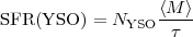
The most common approach for measuring SFRs in resolved regions, such as regions within the Milky Way, is to count individual objects or events (e.g., supernovae) that trace the recent star formation (Chomiuk & Povich 2011). In the molecular clouds within 0.5-1 kpc of the solar system, this is accomplished by counting young stellar objects (YSOs), i.e., protostars at different stages of evolution, which, because they are still embedded in their natal clouds, are optimally identified in the IR. The total number of YSOs is converted to a SFR via:

(1.1)

where the mean YSO mass, < M > depends weakly on the adopted stellar IMF (see Section 1.2.2), and the lifetime of a YSO is, with some uncertainty, ~ 2 Myr (Evans et al. 2009; Heidermann et al. 2010; Gutermuth et al. 2011). The SFR(YSO) is in units of M yr^-1.

In unresolved systems, SFR indicators are merely measures of luminosity, either monochromatic or integrated over some wavelength range, with the goal of targeting continuum or line emission that is sensitive to the short-lived massive stars. The conversion from the luminosity of massive stars to a SFR is performed under the assumption that: (1) the star formation has been roughly constant over the timescale probed by the specific emission being used; (2) the stellar IMF is known (or is a controllable parameter) so that the number of massive stars can be extrapolated to the total number of high+low mass stars formed; and (3) the stellar IMF is fully sampled, meaning that at least one star is formed in the highest-mass bin, and all other mass bins are populated accordingly with one or more stars (see discussion in Section 1.2.2).

SFR indicators in the UV/optical/near-IR range (~ 0.1-5 µm) probe the direct stellar light emerging from galaxies, while SFR indicators in the mid/far-IR ( ~ 5-1000 µm) probe the stellar light reprocessed by dust. In addition to direct or indirect stellar emission, the ionising photon rate, as traced by the gas ionised by massive stars, can be used to define SFR indicators; photo-ionised gas usually dominates over shock-ionised gas in galaxies or large structures within galaxies (e.g., Calzetti et al. 2004; Hong et al. 2011). Tracers include hydrogen recombination lines, from the optical, through the near-IR, all the way to radio wavelengths, forbidden metal lines, and, in the millimetre range, the free-free (Bremsstrahlung) emission. The X-ray emission produced by high-mass X-ray binaries, massive stars, and supernovae can also, in principle, be used to trace SFRs. Finally, the synchrotron emission from galaxies can be calibrated as a SFR indicator (Condon 1992), since cosmic rays are produced and accelerated in supernova remnants, and core-collapse supernovae represent 70% or more of the total supernovae in star-forming galaxies (Bossier & Prantzos 2009).

The following five subsections describe in more detail a few of these SFR indicators for unresolved systems. The emission contribution to the galaxy luminosity from a potential active galactic nuclei (AGN) can be large, depending on the galaxy type and the wavelength of the SFR indicator. I assume that this potential contribution has been recognised and removed from the emission that is being used as a SFR indicator.

1.2.1.1. Indicators based on direct stellar light

The youngest stellar populations emit the bulk of their energy in the restframe UV (< 0.3 µm); in the absence of dust attenuation, this is the wavelength range `par excellence' to investigate star formation in galaxies over timescales of 100-300 Myr, since both O and B stars are brighter in the UV than at longer wavelengths. As a reference, the lifetime of an O6 star is ~ 6 Myr, and that of a B8 star is ~ 350 Myr. The luminosity ratio at 0.16 µm of an O6 to a B8 star is ~ 90, but, if the stellar population follows a Kroupa (2001) IMF (see Section 1.2.2), for every O6 star formed, about 150 B8 stars are formed. Thus, at age zero, the UV emission from the collective contribution of B8 stars is comparable to that of O6 stars.

For a Kroupa stellar IMF, with constant star formation over 100 Myr, the non-ionising UV (0.0912 µm < < 0.3µm) stellar continuum can be converted to a SFR:

(1.2)

with SFR(UV) in M yr^-1, in Å, and L() in erg/s. The stellar SED used for this calibration is from Starburst99, with solar metallicity (Leitherer et al. 1999). The accuracy of the calibration constant is ± 15%, which takes into account small variations as a function of .

For constant star formation over timescales longer than 100 Myr, the calibration constant only decreases by a few percent. However, for shorter timescales, changes are more significant. For = 10 Myr and 2 Myr, the constant is about 42% and a factor 3.45, respectively, higher than in Equation 1.2 (Table 1.1). This shows that if star formation has been active in a region on a timescale shorter than about 100 Myr, the cumulative UV emission of massive stars is still increasing in luminosity, and the calibration of any SFR(UV) indicator has to take this fact into account.

Table 1.1. Model-based luminosity-to-SFR calibrations

Luminositya	Cb	Assumptionsc
L(UV)	3.0 × 10-47	0.1-100 M, 100 Myr
L(UV)	4.2 × 10-47	0.1-30 M, 100 Myr
L(UV)	4.3 × 10-47	0.1-100 M, = 10 Myr
L(UV)	1.0 × 10-46	0.1-100 M, = 2 Myr
L(TIR)	1.6 × 10-44	0.1-100 M, = 10 Gyr
L(TIR)	2.8 × 10-44	0.1-100 M, = 100 Myr
L(TIR)	4.1 × 10-44	0.1-30 M, = 100 Myr
L(TIR)	3.7 × 10-44	0.1-100& M, = 10 Myr
L(TIR)	8.3 × 10-44	0.1-100 M, = 2 Myr
L(H)	5.5 × 10-42	0.1-100 M, 6 Myr, Te = 104 k, ne = 100 cm-3
L(H)	3.1 × 10-41	0.1-30 M, 10 Myr, Te = 104 k, ne = 100 cm-3
L(Br)	5.7 × 10-40	0.1-100 M, 6 Myr, Te = 104 k, ne = 100 cm-3
a Luminosity in erg s-1. Stellar and dust continuum luminosities are given as L(); total IR=TIR is assumed to be equal to the stellar population bolometric luminosity.
b The constant C appears in the calibration as: SFR() =C L(), where SFR is in units of M. The constant is derived from stellar population models, with constant star formation and solar metallicity (Starburst99, Leitherer et al. 1999). For SFR(UV), the numerical value is multiplied by the wavelength in Å.
c Assumptions for mass range of the stellar IMF, which we adopt to have the expression derived by Kroupa (2001), see Section 1.2.2, and for the timescale over which star formation needs to remain constant, for the calibration constant to be applicable. For nebular lines, the adopted values of electron temperature and density are also listed.

As the vast majority of galaxies contain at least some dust, the use of SFR(UV) becomes complicated, since dust attenuation corrections are usually required, and are uncertain. For the most part dust corrections only work on ensembles of systems, rather than individual objects. In a show of Cosmic Conspiracy, the most active and luminous systems are also richer in dust, implying that they require more substantial corrections for the effects of dust attenuation (Wang & Heckman 1996; Calzetti 2001; Hopkins et al. 2001; Sullivan et al. 2001; Calzetti et al. 2007). As a reference number, a modest optical attenuation A_V = 0.9 produces a factor ten reduction in the UV continuum at 0.13 µm, if the attenuation curve follows the recipe of Calzetti et al. (2000).

1.2.1.2.Indicators based on dust-processed stellar light

The IR luminosity of a system will depend not only on its dust content, but also on the heating rate provided by the stars. To first order, the shape of the thermal IR SED will depend on the starlight SED, in the sense that UV-luminous, young stars will heat the dust to higher mean temperatures than old stellar populations (e.g., Helou 1986).

Because of the properties of the Planck function, hotter dust in thermal equilibrium has higher emissivity in the IR than cooler dust. Furthermore, the cross-section of the dust grains for stellar light is higher in the UV than in the optical, as inferred from the typical trend of interstellar extinction curves. Thus, qualitatively, the dust heated by UV-luminous, young stellar populations will produce an IR SED that is more luminous and peaked at shorter wavelengths (observationally 60 µm) than the dust heated by UV-faint, old or low-mass stars (observationally with an IR SED peak at 100-150 µm). This is the foundation for using the IR emission ( ~ 5-1000 µm) as a SFR indicator.

The thermal IR emission is, however, a `blunt tool' for measuring SFRs, in the sense that there is not a one-to-one mapping between UV photons and IR photons, and a monochromatic heating source will produce a modified Planck function for the thermal equilibrium dust emission. Hence the use of `bolometric' IR measures for SFRs, where the IR emission is integrated over the full wavelength range; in practice, most of the emission is located in the wavelength range ~ 5-1000 µm. The bolometric IR luminosity is often indicated with L(TIR) (where TIR is the total infrared emission), and a star formation rate calibration for a stellar population undergoing constant star formation over = 100 Myr is:

(1.3)

with SFR(TIR) in M yr^-1, and L(TIR) in erg/s. For this calculation I have assumed that the Starburst99, Solar-metallicity stellar bolometric emission is completely absorbed and re-emitted by dust, i.e., L_star(bol) = L(TIR).

Not all the stellar emission in a galaxy is generally absorbed by dust. A ballpark number is given by the cosmic background radiation (e.g., Dole et al. 2006), which shows about half of the light emerging at UV-optical-near-IR wavelengths and half at IR wavelengths. Thus, a simplified approach would be to assume that in a typical galaxy only about half of its stellar light is absorbed by dust. This fraction is, however, strongly dependent on the dust content and distribution within the galaxy itself. The application of the SFR(TIR) calibration derived in this section to actual galaxies, which is based on models and the assumption that all of the stellar emission is absorbed by dust and re-emitted in the IR, will therefore result in a lower limit to the true SFR.

The main reason for giving a theoretical expression for SFR(TIR) is to show how dependent the calibration is on assumptions on the stellar population's characteristics. If = 10 Myr and 2 Myr, the calibration constant has -dependent variations that are not too dissimilar from those of SFR(UV) (Table 1.1). However, unlike SFR(UV), the calibration constant of SFR(TIR) keeps changing for star formation timescales longer than 100 Myr, and for = 10 Gyr it is about 57% of the 100 Myr calibration constant. The difference relative to the SFR(UV) case is due to the accumulation over time of long-lived, low-mass stars in the stellar SED. These contribute to the TIR emission, but not to the UV one. The heating of dust by multiple-age stellar populations has the additional effect of producing a thermal equilibrium IR SED that is significantly broader than that produced by a single-temperature modified blackbody function. This has been modelled in the past with at least two approaches: (1) two or more dust components with different temperatures, or (2) one single-temperature dust component with a small absolute value of the dust emissivity index. Physically-motivated models are now available (Draine & Li 2007), which describe the dust emission from galaxies with large accuracy (Draine et al. 2007; Aniano et al. 2012).

Progress over the past ~ 10-20 years in dissecting the various dust components that contribute to the IR SED has helped refining the original simple picture (of which a summary can be found in, e.g., Draine 2003, 2009). Since this chapter is about SFR indicators and not dust properties, I will only summarise the salient traits that connect dust characteristics to wavelength regions in the TIR emission.

The short-wavelength mid-IR range ( ~ 3-20 µm) dust emission arises from a combination of broad emission features, generated by the bending and stretching modes of polycyclic aromatic hydrocarbons (PAHs), and continuum. The latter is due to emission from both single-photon, stochastically-heated small dust grains and thermally emitting hot (T > 150 K) dust: which of these two components dominates depends on the nature of the heating sources, although single-photon heating is predominant in the general interstellar medium of the Milky Way.

The long-wavelength mid-IR range ( ~ 20-60 µm) is emission continuum dominated by hot/warm (T 50 K) dust in thermal equilibrium and single-photon heated small-grain dust. This is the region where, in most galaxies, the dust emission transitions from being dominated by emission from stochastically heated grains to being dominated by large grains in thermal equilibrium.

Finally, the far-IR range ( 60 µm) is mainly due to thermal emission from large grains. The mean temperature of the dust decreases for longer wavelengths (termed `cool' or `cold' dust, depending on the author), although typical temperatures are about 15-20 K or above.

Both massive, short-lived stars and low-mass, long-lived stars can heat the dust contributing to each of the spectral regions identified above. However, UV-bright stars will likely heat the surrounding dust to relatively high effective temperatures. The ~ 20-60 µm IR wavelength region, where the emission transitions from stochastic heating to thermal heating, has thus been targeted as a promising region for defining monochromatic (single-band) SFR indicators. The advantage of such indicators is the ease of use: instead of obtaining multi-point measurements along the IR SED and/or perform uncertain extrapolations, monochromatic IR SFR indicators only require a single wavelength measurement.

Owing to the uncertainty of assigning a given waveband to a specific dust emission component, monochromatic IR SFRs have been calibrated across a wide range of IR wavelengths, including the IR Space Observatory (ISO) 7 and 15 µm bands, the Spitzer Space Telescope 8, 24, 70 µm bands, and, currently, the Herschel Space Telescope 70 µm and longer wavelength bands. The range of angular resolutions offered by each facility has been and is enabling the calibration of both global and local SFR indicators.

Monochromatic SFR indicators shortward of 15-20 µm require care of use: stochastically-heated dust can trace both young and evolved stellar populations (e.g., Boselli et al. 2004; Calzetti et al. 2007; Bendo et al. 2008; Crocker et al. 2012). The PAHs may be better tracers of B stars than current SFR (Peeters et al. 2004), and the emission features show strong dependence on the metal abundance of the system (e.g., Madden et al. 2000, 2006; Engelbracht et al. 2005, 2008; Draine et al. 2007; Smith et al. 2006; Galliano et al. 2008; Gordon et al. 2008; Muñoz-Mateos et al. 2009; Marble et al. 2010). Only about 50% of the emission at 8 µm from a galaxy is dust-heated by stellar populations 10 Myr or younger, and about 2/3 by stellar populations 100 Myr or younger (Crocker et al. 2012). Thus, a significant fraction of the 8 µm emission is unrelated to current star formation. While this is likely to affect mainly studies of sub-galactic regions or structures, some effect may be expected on the global SFR indicators. Various calibration efforts have usually recovered a roughly linear or slightly sub-linear relation between the global 8 µm luminosity, providing reference SFR indicators for metal-rich, star-forming galaxies. However, the peak-to-peak scatter tends to be large, a factor of about three (Treyer et al. 2010), with larger deviations observed for compact starbursts (Elbaz et al. 2011).

Longward of around 70 µm, the contribution to the IR SED of thermal dust at increasingly lower temperature, and therefore heated by stars that are low-mass and long-lived, becomes more and more prominent, thus compromising the ability of the IR emission to trace exclusively or almost exclusively recent star formation.

For the above two reasons, I offer here only two empirical monochromatic IR SFR calibrations: in the 24 µm and 70 µm restframe bands. I distinguish between local and global SFR indicators, since, as discussed earlier in this section, the bolometric luminosity of a stellar population undergoing constant star formation increases with time. Therefore, to the extent that the IR emission traces the bolometric emission of the stellar population, the calibration constant will be different for a global, galaxy-wide SFR indicator and a local SFR indicator, since the former includes the Hubble-time-integrated stellar population of a galaxy, while the latter is generally derived from regions that are dominated by stellar populations with short star formation timescales (Hii regions, large star-forming complexes, etc.).

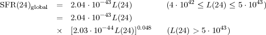
At 24 µm, the local (spatial scale ~ 500 pc) calibration offered by Calzetti et al. (2007) is:

(1.4)

with SFR(24) in M yr^-1, and L(24) = L() in erg s^-1. The uncertainty is 0.02 in the exponent, and 15% in the calibration constant. The non-linear correlation between L(24) and SFR is a common characteristic of this tracer at the local scale (Alonso-Herrero et al. 2006; Pérez-González et al. 2006; Calzetti et al. 2007; Relaño et al. 2007; Murphy et al. 2011), and may be a manifestation of the increasing transparency of regions for decreasing L(24) luminosity, of the increasing mean dust temperature for increasing L(24) luminosity, or a combination of the two.

At the galaxy-wide scale, both linear and non-linear correlations between SFR and L(24) have been derived (Wu et al. 2005; Zhu et al. 2008; Kennicutt et al. 2009; Rieke et al. 2009), perhaps owing to differences in sample selections and in the reference SFR indicators used to calibrate SFR(24), and sufficient scatter in the data that both linear and non-linear fits can be accommodated (Wu et al. 2005; Zhu et al. 2008). The linear calibration of Rieke et al. (2009), reported using the same IMF as all the other indicators in this presentation, is:

(1.5)

where a small correction for self-absorption is included at the high luminosities. The linear calibrations in the literature tend to be within 30% of each other, suggesting a general agreement.

At 70 µm, the local calibration over ~ 1 kpc scales derived by Li et al. (2010) using over 500 star-forming regions is:

(1.6)

with SFR(70) in M yr^-1, and L(70) = L() in erg s^-1. The formal uncertainty on the calibration constant is about 2%, although the scatter in the datapoints is about 35%. The global calibration provided by Calzetti et al. (2010) is:

(1.7)

with a scatter of the datapoints of about 60%. The SFR(70) calibration constant thus increases when going from whole galaxies to 1 kpc regions, i.e., for decreasing region sizes. Li et al. (2012) obtain a tantalising result: the calibration constant for SFR(70) becomes even larger for regions smaller than ~ 1 kpc. These constants can be interpreted in terms of star formation timescale within each region size (Fig. 1.1), for simple assumptions on the star formation history, the fraction of stellar light re-emitted by dust in the IR, and the fraction of IR emission contained in the 70 µm band (Draine & Li 2007).

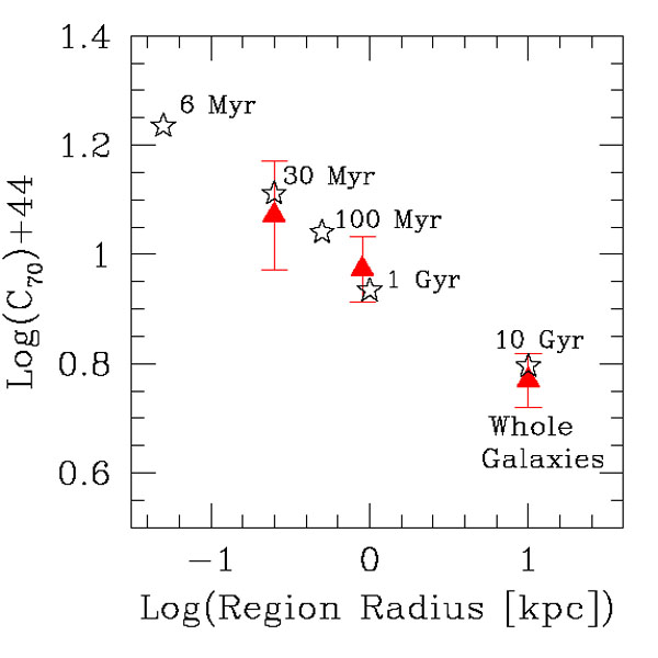Figure 1.1. The calibration constant, C70, between SFR and the 70 µm luminosity, expressed as SFR(70) = C70 L(70), as a function of the physical size of the regions used to derive the calibration. The filled red triangles are observed values from Li et al. (2010, 2012) and Calzetti et al. (2010), using both Spitzer and Herschel data. The black stars are from stellar population synthesis models, for constant star formation and a Kroupa IMF, in the stellar mass range 0.1-100 M; the mean age of the population that best approximates the observed C70 values is shown. The scaling between bolometric light and 70 µm emission is discussed in Calzetti et al. (2010). The association between star formation timescale and region size is based on a region crossing time with a 1-3 km s-1 speed.

Gas-rich, but metal-poor, galaxies offer little opacity to stellar emission (the same is true for metal-rich, but gas-poor galaxies, e.g., ellipticals, but for these galaxies few or no stars form). Metal content correlates with galaxy luminosity (Tremonti et al. 2004, and references therein), and faint galaxies are faint IR emitters. In this case, SFR(IR) becomes a highly uncertain tool. SFR tracers that mix tracers of both dust-obscured and dust-unobscured star formation have recently been calibrated, and will be presented in Section 1.2.1.4.

1.2.1.3. Indicators based on ionised gas emission

Young, massive stars produce copious amounts of ionising photons that ionise the surrounding gas. Hydrogen recombination cascades produce line emission, including the well-known Balmer series lines of H (0.6563 µm) and H (0.4861 µm), which, by virtue of being strong and located in the optical wavelength range, represent the most traditional SFR indicators (Kennicutt 1998).

Only stars more massive than ~ 20 M produce a measurable ionising photon flux. In a stellar population formed through an instantaneous burst with a Kroupa IMF the ionising photon flux decreases by two orders of magnitude between 5 Myr and 10 Myr after the burst.

The relation between the intensity of a hydrogen recombination line and the ionising photon rate is dictated by quantum mechanics, for a nebula that is optically thick to ionising photons (case B, Osterbrock & Ferland 2006). Case B is usually assumed for most astrophysical situations where SFRs are of interest. Although typical interstellar hydrogen densities are sufficient to ensure that most Hii regions should be radiation-bound, inhomogeneities in the interstellar medium cause some fraction of the ionising photons to leak out of the regions (but usually not out of galaxies). More discussion on this issue is given below. The relation between the luminosity of the H emission line and the ionising photon rate is given by Osterbrock & Ferland (2006):

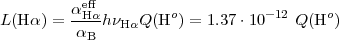(1.8)

where L(H) is in erg s^-1, _H^eff is the effective recombination coefficient at H, _B is the case B recombination coefficient, Q(H^o) is the ionising photon rate in units of s^-1, and the constant at the right-hand side of the equation is the resulting coefficient for electron temperature T_e = 10000 K and density n_e = 100 cm^-3. For a Kroupa IMF (Section 1.2.2), the relation between ionising photon rate and SFR is:

(1.9)

with SFR(Q(H^o)) in M yr^-1. Combining Equations 1.8 and 1.9, we obtain the well-known calibration:

(1.10)

again, with SFR(H) in M yr^-1 and L(H) in erg s^-1. The variation of the calibration constant is ~ 15% for variations in electron temperature in the range T_e = 5000-20000 K , and is < 1% for electron density variations in the range n_e = 100-10⁶ cm^-3 (Osterbrock & Ferland 2006). Star formation needs to have remained constant over timescales > 6 Myr for the calibration constant to be applicable (Table 1.1), but there is no dependency on long timescales, unlike SFR(UV) or SFR(TIR).

All SFR indicators that use the ionisation of hydrogen to trace the formation of massive stars are sensitive to the effects of dust. The most commonly treated effect is that of dust attenuation of the line or continuum. As we will see in Section 1.4, various techniques have been developed to try to remove this effect; furthermore, dust attenuation decreases for increasing wavelength. A far more difficult effect to treat is the direct absorption of Lyman continuum photons by dust. In this case, the ionising photons are removed altogether from the light beam and are no longer available to ionise hydrogen. Thus, no emission from either recombination lines or free-free continuum emission will result. The actual impact of Lyman continuum photon (Lyc) absorption by dust has been notoriously difficult to establish from an empirical point of view, owing to the absence of a `ground truth' (or reference) with which to compare measurements. Models have to be involved, and these show that the level of Lyc absorption depends on the assumption for the geometry of the nebulae (Dopita et al. 2003, and references therein). The parametrisation of Dopita et al., where the ratio of H line luminosity with and without Lyc absorption is given as a function of the product of metal abundance and ionisation parameter, shows that most normal disk galaxies fall into the regime of low Lyc absorption, typically less than 15%-20%; however, Lyc absorption by dust can become significant at large ionisation parameters and metallicities, such as those typical of local luminous and ultra-luminous IR galaxies (LIRGs and ULIRGs, galaxies with bolometric luminosity > a few 10¹¹ L), and of some high-density central regions of galaxies.

A somewhat opposite effect is represented by leakage of ionising photons, i.e., case B recombination does not fully apply. Leakage of ionising photons from galaxies is likely negligible, at the level of a few percent or less (e.g., Heckman et al. 2011), although the jury is still out in the case of low-mass, low-density galaxies (Hunter et al. 2010; Pellegrini et al. 2012). Star-forming regions within galaxies tend, on the other hand, to be leaky, and lose about 25%-40% of their ionising photons (see recent work by Pellegrini et al. 2012; Relaño et al. 2012; Crocker et al. 2012). Thus, the use of ionising photon tracers for local SFRs may be biased downwards by about 1/3 of their true value because of this effect. This correction is not included in Table 1.1.

Adopting for the moment that Lyc absorption by dust and leakage are not issues, emission lines still need to be corrected for the effects of dust attenuation. As an example, a modest attenuation of A_V = 1 mag by foreground dust depresses the H luminosity by a factor ~ 2. At longer wavelengths, Br (2.16 µm) is depressed by only 11%, for the same A_V. Recent advances in the linearity, stability, and field-of-view size of infrared detectors' are making it possible to collect significant samples of galaxies observed in the IR Hydrogen recombination lines. Table 1.1 shows a calibration for Br, derived under the same assumptions as SFR(H). Calibrations for other lines can be inferred from those of H and Br and the emissivity ratios published in Osterbrock & Ferland (2006).

Recombination lines at wavelengths longer than the optical regime, while offering the advantage of lower sensitivity to dust attenuation, have the dual disadvantage of being progressively fainter and more sensitive to the physical conditions of the gas, especially the temperature; these are natural consequences of transition probabilities and conditions of thermal equilibrium, respectively. The luminosity of Br is about 1/100th of that at H, and it changes by about 35% for T_e in the range 5000-20000 K, and by ~ 4% for density in the range n_e = 10²-10⁶ cm^-3. For Br (4.05 µm), the variations are 58% and 13% for changes in T_e and n_e, respectively. The sensitivity of Br and Br to T_e is a factor 2.4 and 3.9 larger, respectively, than that of L(H).

New or greatly improved radio and millimetre facilities such as ALMA (the Atacama Large Millimetre/submillimetre Array) or EVLA (the Expanded Very Large Array) are opening the window for exploring millimetre and/or radio recombination lines as ways to measure SFRs unimpeded by effects of dust attenuation, albeit using lines that are intrinsically extremely weak. I will cumulatively refer as RRLs all (sub)millimetre and radio recombination lines from hydrogen quantum levels n > 20. At high quantum numbers (n > 80-200, depending on electron density), i.e., at wavelengths of a few cm or longer, stimulated emission is no longer negligible and adds extra parameters in the expression of the line luminosity (Brown et al. 1978). Even within the regime where stimulated emission is not a concern, the line luminosity is dependent on the electron temperature, producing SFR(RRL) T_e^0.7 (Gordon & Sorochenko 2009). This translates into a variation in the line intensity of a factor 2.6 for T_e in the range 5000-20000 K.

The traditional approach of measuring the electron temperature from the radio line-to-continuum ratio relies on the assumption that the underlying continuum is free-free emission. The true level of free-free emission from a galaxy, or from a large star-forming region embedded in a galaxy, needs to be carefully disentangled from both dust emission (dominant < 2-3 mm) and synchrotron emission (dominant > 1-3 cm, depending on the source). Often, multi-wavelength observations are used to accomplish this (e.g., Murphy et al. 2011), and add an additional layer of complication to the use of SFR(RRL). Exploratory work is still ongoing to test how efficiently RRLs can be detected in external galaxies (e.g., Kepley et al. 2011), and what advantage they can bring relative to more classical and efficient methods. If the high-density, and heavily dust-obscured, regime turns out to be the main niche for these tracers (Yun 2008), they will need to be carefully weighted against SFR(IR), in light of the potentially heavy impact of the Lyc absorption by dust.

The free-free emission from galaxies or regions itself is a SFR tracer, being the product of the Coulomb interaction between free electrons and ions in thermal equilibrium. The electron temperature dependence of this SFR tracer, SFR(ff) T_e^-0.45 (Condon 1992), is shallower than that of the SFR(RRL), implying less than a factor of two change for a factor of four variation in T_e. A calibration of SFR(ff) consistent with our IMF choice is given in Murphy et al. (2011).

SFR tracers that use forbidden metal line emission will not be discussed in this review, as they suffer from the same limitations as the hydrogen recombination lines, and have additional dependencies on the metal content and ionisation conditions of a galaxy or region. A review is found in Kennicutt (1998) and a recent calibration in Kennicutt et al. (2009).

1.2.1.4. Indicators based on mixed processes

The necessity to capture both dust-obscured and dust-unobscured star formation has led to the formulation of SFR indicators that attempt to use the best qualities of each indicator above. This advantage compensates for the slight disadvantage of having to obtain two measures at, generally, two widely separated wavelengths: one that measures the direct stellar light and one that measures the dust-processed light. These mixed indicators have been calibrated empirically over the past ~ 5-7 years, using combinations of data from space and the ground (e.g., Calzetti et al. 2005, 2007; Kennicutt et al. 2007, 2009; Liu et al. 2011; Hao et al. 2011), and are usually expressed as:

(1.11)

with SFR(₁, ₂) in M yr^-1. ₁ is usually a wavelength probing either direct stellar light (e.g., the GALEX FUV at 0.153 µm) or ionised gas tracers (e.g., H), and ₂ is a wavelength or range of wavelengths where dust emission dominates (e.g., 24 µm, 25 µm, TIR, etc.). The constant C(₁) is the calibration for the direct stellar light probe, often derived from models (see Table 1.1). The luminosities L(₁)_obs and L(₂)_obs are in units of erg s^-1 and are the observed luminosities (i.e., not corrected for effects of dust attenuation or other effects). The proportionality constant a_{2, Type} depends on both the dust emission tracer used and whether the calibration is for local or global use (Type = local, global). This latter characteristic is due to the sensitivity of dust emission to heating from a wide range of stellar populations (see Section 1.2.1.2). An example of a mixed indicator calibration is given in Fig. 1.2.

Figure 2. An example of the calibration for a mixed SFR indicator, from Calzetti et al. (2007). This specific example is for a local SFR indicator: the data points include star-forming regions in nearby galaxies (red triangles, green squares, blue crosses) and local LIRGs (black stars, from Alonso-Herrero et al. 2006). The horizontal axis is the luminosity/area of the regions/galaxies in the hydrogen recombination line P (1.8756 µm), the vertical axis is a linear combination of the luminosity/area of the observed H and 24 µm luminosity. The star-forming regions include low (blue), intermediate (green), and high (red) metallicity. All the points align basically along a one-to-one relation (straight continuous line) suggesting that this calibration is fairly independent of the metallicity (dust content) and luminosity of the source. Other lines mark the position of models as described in Calzetti et al. (2007).

Table 1.2 summarises a few of the published calibrations from the references above; a more complete set of global calibrations can be found in the recent review by Kennicutt & Evans (2012). Local calibrations show systematically higher values of a_{2, Type} than global ones. At 24-25 µm, a_{24, local} / a_25,global ~ 1.55. This difference cannot be attributed to the difference between L(24) and L(25), which is around 2% typically (Kennicutt et al. 2009; Calzetti et al. 2010). The larger fraction of 24 µm emission that needs to be added to either FUV or H in local SFR measurements may simply reflect the fact that regions within galaxies are probing stellar populations over shorter timescales ( ~ 100 Myr or smaller) than global SFR measurements ( > many Gyr). The dust emission traces this difference accordingly (Kennicutt et al. 2009). From Table 1.1, the ratio of the calibration constants for SFR(TIR) at 100 Myr and 10 Gyr is 1.75, close to the observed value of 1.55. Differences in the mean dust temperature, that is likely to boost the L(24) in sub-galactic regions, may account for the remaining discrepancy.

Table 1.2. Mixed processes-based SFR calibrations ^a

1b	2b	C1c	a2,Typed	Typed
FUV (0.153 µm)	24 µm	4.6 × 10-44	6.0	local
FUV (0.153 µm)	25 µm	4.6 × 10-44	3.89	global
FUV (0.153 µm)	TIR	4.6 × 10-44	0.46	global
H	24 µm	5.5 × 10-42	0.031	local
H	25 µm	5.5 × 10-42	0.020	global
H	TIR	5.5 × 10-42	0.0024	global
a The calibrations are expressed as: SFR(1, 2) = C(1) [L(1)obs + a2, Type L(2)obs], see text. The SFR is in units of M yr-1. The luminosities L(1)obs and L(2)obs are in units of erg s-1 and are the observed luminosities. Stellar or dust continuum luminosities are given as L(); TIR is the dust luminosity integrated in the range ~ 5-1000 µm (e.g., Dale & Helou 2002). The calibration constants are from: Calzetti et al. 2005, 2007; Kennicutt et al. 2007, 2009; Liu et al. 2011; Hao et al. 2011.
b 1 is centred in the GALEX FUV at 0.153 µm or at H, and 2 is 24 µm, 25 µm, or TIR. The difference in luminosity between 24 µm and 25 µm is around 2% (Kennicutt et al. 2009; Calzetti et al. 2010).
c The constant C(1) is the calibration for the direct stellar light probe, derived from models or empirically. In this Table, we adopt model-derived values (Table 1.1).
d The constant a2, Type provides the fraction of dust-processed light at 2 that needs to be added to the direct stellar/gas probe at 1. `Type' refers to either a local calibration (applicable to regions in galaxies 0.5-1 kpc) or a global calibration (whole galaxies).

1.2.1.5. Indicators based on other processes

SFR indicators based on non-thermal (synchrotron) radio and X-ray emission represent more indirect ways of probing star formation in galaxies.

In the case of synchrotron emission, the basic mechanism is the production and acceleration of cosmic rays in supernova explosions; since the supernova rate is directly related to the SFR, we should be able to use the synchrotron luminosity as a proxy for the SFR. There is, however, an added complication in that the non-thermal luminosity depends not only on the mean cosmic ray production per supernova, but also on the galaxy's magnetic field (e.g., Rybicki & Lightman 2004). The case for SFR(sync) is helped by the well-known IR-radio correlation (e.g., Yun et al. 2001): if the IR is correlated with both SFR and radio emission, then SFR and radio emission are correlated among themselves. SFR(sync) calibrations can only be derived empirically (Condon 1992; Schmitt et al. 2006; Murphy et al. 2011), because of the complexity of the relation between the SFR and the underlying physical mechanism; a recent derivation consistent with our IMF can be found in Murphy (2011).

A similarly indirect relation exists between SFR and X-ray luminosity. In star-forming galaxies, the X-ray luminosity is produced by high-mass X-ray binaries, massive stars, and supernovae, but non-negligible contributions from low-mass X-ray binaries are also present. The latter are not directly related to recent star formation, and represent a source of uncertainty in the calibration of SFR(X-ray). Because of the difficulty of establishing the frequency and intrinsic luminosity of each X-ray source (related or unrelated to current star formation) from first principles, the SFR(X-ray) calibrations have been derived empirically, and examples are given in Ranalli et al. (2003), Persic & Raphaeli (2007), and Mineo et al. (2012). Care should be taken when comparing these published calibrations, obtained for a Salpeter IMF, with those reported in this summary, which are based on a Kroupa IMF.

1.2.2. A word about the stellar initial mass function and stochastic sampling

All calibrations listed in this section make the implicit assumption that the stellar IMF is constant across all environments and given by the double-power law expression (Kroupa 2001):

(1.12)

where (M) is the number of stars between M and M + dM. The stellar mass distribution and total stellar mass produced by this expression are not significantly different from that produced by the log-normal expression proposed by Chabrier (2003). The Kroupa IMF expression produces a smaller number of low-mass stars than the Salpeter (1955) IMF, which has been customarily represented with a single power law with slope -2.35 between 0.1 and 100 M. Since the majority of SFR indicators trace massive stars, a calibration based on the Kroupa IMF can be converted to one using the Salpeter IMF simply by multiplying the calibration constant by 1.6.

The assumption that the IMF is constant and universal is justified by many observational results, although these are generally rather uncertain, especially at the high-mass end (review by Bastian et al. 2010). There is still the possibility of variation in some extreme (in terms of density, SFR, or other) environments, and arguments both in favour of and against variations have been brought forward by many different authors. To gauge the impact of a different IMF assumption on our SFR calibrations, we can adopt a modified Kroupa IMF, with the maximum stellar mass set to 30 M, instead of 100 M. The new calibration constants, for selected timescales, are listed in Table 1.1. The constants change by factors 1.4, 1.5, and 5.6 for SFR(UV), SFR(TIR), and SFR(H), respectively. The change for the H calibration is the largest of all; it is larger than the UV one by a factor of four, simply because significant UV emission is produced by stars down to ~ 5 M, but significant ionising photon flux is produced only by stars more massive than ~ 20 M. In addition, it takes slightly longer (10 Myr for the upper mass limit of 30 M versus 6 Myr for 100 M) for the ionising photons to reach their asymptotic value. The changes for the UV and TIR calibration constants are similar to each other.

In contrast with the results just discussed, the mean stellar mass for the Kroupa IMF is < M > ~ 0.6 M, with less than 10% difference between using 100 M or 30 M as stellar upper mass limit. This makes tracers based on the mean stellar mass of a system (Equation 1.1) more robust than those based on tracing the most massive stars.

Even if the IMF is universal, individual systems may show departures from this condition, based on simple arguments of sampling.

If we consider a single-age, very young stellar cluster, we can ask what the minimum mass is that this cluster needs to have so that at least one star with mass 100 M is formed. The mass is 2.8 × 10⁵ M, which is a large value, only achieved by some of the most massive star clusters known. As a comparison, if the maximum stellar mass is 30 M, full sampling of the IMF, meaning that at least one 30 M star is formed, is achieved with a cluster mass of 1.7 × 10⁴ M.

Under these circumstances, it is not uncommon that studies that involve low SFRs, either because the region considered is small and/or inefficient at forming stars, or because the galaxy has a low overall SFR, are subject to the effects of stochastic sampling, i.e., the stellar IMF is randomly, not fully, sampled. The impact of stochastic sampling is higher for the most massive stars, since there are proportionally less massive stars than low-mass ones. From the Kroupa IMF expression above, only 11% of all stars, by number, have masses above 1 M, although these stars represent 56% of the total mass.

Stochastic sampling has a larger impact on tracers of ionising photons than on tracers of UV continuum light, for the same reason that a low upper limit in stellar mass has. Clear evidence for this is shown by the so-called extended UV (XUV) disks of galaxies, as revealed by GALEX. The original hypothesis that these XUV disks, bright in the UV but faint in H, could be due to peculiar IMFs (e.g., deficient in high-mass stars) has been replaced by the finding that the IMF is stochastically sampled in these low-SFR areas (Goddard et al 2010; Koda et al. 2012). The models of Cerviño et al. (2002), renormalised to the Kroupa IMF (Equation 1.12), show that a star cluster with mass ~ 1 × 10⁴ M will be subject to sufficient stochastic sampling that a scatter as large as 20% can be expected in the measured ionising photon flux. The scatter increases dramatically for decreasing cluster mass, and becomes as large as 70% for a cluster mass ~ 1 × 10³ M. This poses a practical limitation of SFR 0.001 M yr^-1 for the use of SFR indicators based on the ionising photon flux if a 20% or less uncertainty is desired; a similar uncertainty value for the UV is obtained at SFR 0.0003 M yr^-1, or about 3.5 times lower than when using tracers of ionising photons (Lee et al. 2009, 2011).