Annu. Rev. Astron. Astrophys. 2013. 51: 207-268 Copyright © 2013 by Annual Reviews. All rights reserved

4. X_CO IN THE MILKY WAY

The Galaxy is the only source where it is possible to determine the CO-to-H₂ conversion factor in a variety of ways. It thus provides the prime laboratory to investigate the calibration and the variations of the proportionality between CO emission and molecular mass.

In the following sections we will discuss three types of X_CO determinations: 1) employing virial masses, a technique that requires the ability to spatially resolve molecular clouds to measure their sizes and kinematics, 2) taking advantage of optically thin tracers of column density, such as dust or certain molecular and atomic lines, and 3) using the diffuse -ray emission arising from the pion production process that takes place when cosmic rays interact with interstellar medium protons. Gamma-ray techniques are severely limited by sensitivity, and are only applicable to the Milky Way and the Magellanic Clouds. The good level of agreement between these approaches in our own galaxy is the foundation of the use of the CO-to-H₂ conversion factor in other galaxies.

4.1. X_CO Based on Virial Techniques

The application of the virial theorem to molecular clouds has been discussed by a number of authors, and recently reviewed by McKee & Ostriker (2007). Here we just briefly summarize the fundamental points. The virial theorem can be expressed in the Lagrangian (fixed mass) or Eulerian (fixed volume) forms, the latter particularly applicable to turbulent clouds where mass is constantly exchanged with the surrounding medium. In the somewhat simpler Lagrangian form, the virial equilibrium equation is

(20)

where K is the volume integral of the thermal plus kinetic energy, K_s is the surface pressure term, B is the net magnetic energy including volume and surface terms (which cancel for a completely uniform magnetic field), and W is the net gravitational energy which is determined by the self-generated gravitational potential if the acceleration due to mass external to the cloud can be neglected. In the simple case of a uniform, unmagnetized sphere virial equilibrium implies 2K + W = 0. It is useful to define the virial parameter, a_vir, which corresponds to the ratio of total kinetic energy to gravitational energy (Bertoldi & McKee 1992), so that a_vir 5 R² / GM.

4.1.1. Are Clouds Virialized?

In this context, gravitationally bound objects have a_vir ≃ 1. Whether interstellar clouds are entities in virial equilibrium, even in a time or ensemble averaged sense (McKee 1999), is a matter of current debate. Observational evidence can be interpreted in terms of systems out of equilibrium with rapid star formation and subsequent disruption in a few Myr (e.g., Elmegreen 2000), an evolutionary progression and a typical lifetime of a few tens of Myr, long enough for clouds to become virialized (e.g., Blitz & Shu 1980b, Fukui & Kawamura 2010), or a lifetime of hundreds of Myr (e.g., Scoville & Hersh 1979). Roman-Duval et al. (2010) find a median a_vir 0.5 for clouds in the inner Galaxy, suggesting that they are bound entities where M_vir represents a reasonable measure of the molecular mass, although casting doubt on the assumption of exact virial equilibrium. Wong et al. (2011) estimate a very large scatter in a_vir in the Large Magellanic Cloud, but do lack an independent mass tracer so their results rest on the assumption of a fixed X_CO. Observations in the outer Galaxy show another angle of the situation. Heyer, Carpenter & Snell (2001) find that clouds with M_mol > 10⁴ M are self-gravitating, while small clouds with masses M_mol < 10³ M are overpressured with respect to their self-gravity, that is, have a_vir ≫ 1 and are out of equilibrium. Given the observed mass function, however, such clouds represent a very small fraction of the molecular mass of the Milky Way.

In any case, observed GMC properties can be understood as a consequence of approximate energy equipartition, which observationally is very difficult to distinguish from virial equilibrium (Ballesteros-Paredes 2006). Clouds with an excess of kinetic energy, a_vir ≫ 1, perhaps due to ongoing star formation or SNe would be rapidly dissipated, while clouds with a dearth of kinetic energy, a_vir ≪ 1, would collapse at the free-fall velocity which is within 40% of the equipartition velocity dispersion and challenging to distinguish from turbulent motions in observations. Furthermore, the resulting star formation will inject energy into the cloud acting to restore the balance. Thus from the standpoint of determining cloud masses over large samples, the assumption of virial equilibrium even if not strictly correct, is unlikely to be very wrong.

4.1.2. Observational Results

The most significant study of the relation between virial mass and L_CO (the mass-luminosity relation) in the Milky Way is that by Solomon et al. (1987), which encompasses 273 clouds and spans several orders of magnitude in cloud luminosity and mass. It is dominated by clouds located in the inner Galaxy, in the region of the so-called Molecular Ring, a feature in the molecular surface density of the Milky Way peaking at R_GC 4 kpc galactocentric radius. It uses kinematic distances with an old value of the distance to the Galactic Center, R = 10 kpc. We report new fits after a 0.85 scaling in all distances and sizes and 0.72 in luminosities to bring them into agreement with the modern distance scale (R = 8.5 kpc). The virial mass computations assume a (r) r^-1 (see Section 2.1).

Solomon et al. (1987) find a very strong correlation between M_vir and L_CO, such that M_vir = 37.9 L_CO^0.82 with a typical dispersion of 0.11 dex for M_vir. Note the excellent agreement with the expected mass-luminosity relation in Eq. 10 using a typical CO brightness temperature T_B 4 K (Maloney 1990). For a cloud at their approximate median luminosity, L_CO 10⁵ K km s^-1 pc², this yields _CO = 4.6 M (K km s^-1 pc²)^-1 and X_CO,20 = 2.1. Because the relation is not strictly linear _CO will change by ~ 60% for an order of magnitude change in luminosity (Fig. 2). Therefore GMCs with lower luminosities (and masses) will have somewhat larger mass-to-light ratios and conversion factors than more luminous GMCs.

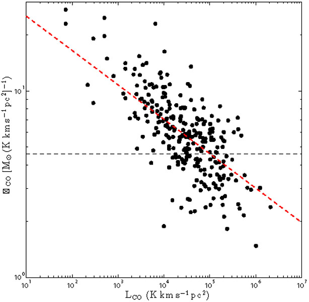Figure 2. Relation between virial CO and CO luminosity for GMCs in the Milky Way (Solomon et al. 1987). We have corrected the numbers in the original table to reflect the updated distance to the Galactic Center of 8.5 kpc. The dependence of CO on LCO arises from the fact that the correlation between Mvir and LCO has a nonlinear slope (Mvir LCO0.815±0.013), following the expectations from Eq. 10 for approximately constant brightness temperature. This results in CO 4.61 (LCO/105)-0.185, denoted by the red thick dashed line (the dispersion around this relation is ± 0.15 dex). The nominal value at LCO = 105 K km s-1 pc2 is illustrated by the thin black dashed line.

Independent analysis using the same survey by Scoville et al. (1987) yields a very similar mass-luminosity relation. After accounting for the different coefficients used for the calculation of the virial mass, the relation is M_vir = 33.5 L_CO^0.85. For a L_CO 10⁵ K km s^-1 pc² cloud this yields _CO = 6.0 M (K km s^-1 pc²)^-1 and X_CO,20 = 2.8 (this work uses R = 8.5 kpc). Interestingly, there is no substantial difference in the mass-luminosity relation for GMCs with or without HII regions (Scoville & Good 1989), although the latter tend to be smaller and lower mass, and have on average half of the velocity-integrated CO brightness of their strongly star-forming counterparts. The resulting difference in T_B could have led to a displacement in the relation, according to the simple reasoning leading to Eq. 10, but it appears not to be significant.

4.1.3. Considerations and Limitations

Besides the already discussed applicability of the virial theorem, there are a number of limitations to virial studies. Some are practical, while others are fundamental to the virial technique. On the practical side, virial studies are sensitive to cloud definitions and biases induced by signal-to-noise. These will impact both the values of R and used to compute the mass. In noise-free measurements isolated cloud boundaries would be defined using contours of zero emission, when in reality it is necessary to define them using a higher contour (for example, Solomon et al. 1987 use a T_B ~ 4 K CO brightness contour). Scoville et al. (1987) discuss the impact of this correction, studying the "curve of growth" for R and as the definition contour is changed in high signal-to-noise observations. Moreover, isolated clouds are rare and it is commonly necessary to disentangle many partially blended features along the line of sight. To measure a size clouds need to be resolved, and if appropriate the telescope beam size needs to be deconvolved to establish the intrinsic cloud size. This is a major concern in extragalactic studies, but even Galactic datasets are frequently undersampled which affects the reliability of the R and L_CO determinations. Given these considerations, it is encouraging that two comprehensive studies using independent analysis of the same survey come to values of _CO that differ by only ~ 30% for clouds of the same luminosity.

A fundamental limitation of the virial technique is that CO needs to accurately sample the full potential and size of the cloud. For example, if because of photodissociation or other chemistry CO is either weak or absent from certain regions, its velocity dispersion may not accurately reflect the mass of the cloud. This is a particular concern for virial measurements in low metallicity regions (see Section 6), although most likely it is not a limitation in the aforementioned determinations of X_CO in the inner Galaxy.

4.2. Column Density Determinations Using Dust and Optically Thin Lines

Perhaps the most direct approach to determining the H₂ column density is to employ an optically thin tracer. This tracer can be a transition of a rare CO isotopologue or other chemical species (e.g., CH Magnani et al. 2003). It can also be dust, usually optically thin in emission at far-infrared wavelengths, and used in absorption through stellar extinction studies.

4.2.1. CO Isotopologues

A commonly used isotopologue is ¹³CO. Its abundance relative to ¹²CO is down by a factor approaching the ¹²C / ¹³C 69 isotopic ratio at the solar circle (¹²C/¹³C 50 at R_GC 4 kpc, the galactocentric radius of the Molecular Ring) as long as chemical fractionation and selective photodissociation effects can be neglected (Wilson 1999). Given this abundance ratio and under the conditions in a dark molecular cloud ¹³CO emission may not always be optically thin, as ₁ ~ 1 requires A_V ~ 5.

The procedure consists of inverting the observed intensity of the optically thin tracer to obtain its column (or surface) density. In the case of isotopologues, this column density is converted to the density of CO using the (approximate) isotopic ratio. Inverting the observed intensity requires knowing the density and temperature structure along the line of sight, which is a difficult problem. If many rotational transitions of the same isotopologue are observed, it is possible to model the line of sight column density using a number of density and temperature components. In practice an approximation commonly used is local thermodynamic equilibrium (LTE), the assumption that a single excitation temperature describes the population distribution among the possible levels along the line of sight. It is also frequently assumed that ¹²CO and ¹³CO share the same T_ex, which is particularly justifiable if collisions dominate the excitation (T_ex = T_kin, the kinetic temperature of the gas). Commonly used expressions for determining N(¹³CO) under these assumptions can be found in, for example, Pineda et al. (2010). Note, however, that if radiative trapping plays an important role in the excitation of ¹²CO, T_ex for ¹³CO will generally be lower due to its reduced optical depth (e.g., Scoville & Sanders 1987b).

Dickman (1978) characterized the CO column density in over 100 lines of sight toward 38 dark clouds, focusing on regions where the LTE assumption is unlikely to introduce large errors. The combination of LTE column densities with estimates of A_V performed using star counts yields A_V (4.0 ± 2.0) × 10^-16 N(¹³CO) cm² mag. Comparable results were obtained in detailed studies of Taurus by Frerking, Langer & Wilson (1982, note the nonlinearity in their expression) and Perseus by Pineda, Caselli & Goodman (2008), the latter using a sophisticated extinction determination (Lombardi & Alves 2001). Extinction can be converted into molecular column density, through the assumption of an effective gas-to-dust ratio. Bohlin, Savage & Drake (1978) determined a relation between column density and reddening (selective extinction) such that [N(HI) + 2N(H₂)] / E(B - V) 5.8 × 10²¹ atoms cm^-2 mag^-1 in a survey of interstellar Ly absorption carried out using the Copernicus satellite toward 75 lines of sight, mostly dominated by HI. For a "standard" Galactic interstellar extinction curve with R_V A_V / E(B - V) = 3.1, this results in

(21)

A much more recent study using Far Ultraviolet Spectroscopic Explorer observations finds essentially the same relation (Rachford et al. 2009). In high surface density molecular gas R_V may be closer to 5.5 (Chapman et al. 2009), and Eq. 21 may yield a 40% overestimate (Evans et al. 2009). Using Eq. 21, the approximate relation between ¹³CO J = 1 → 0 and molecular column density is N(H₂) 3.8 × 10⁵ N(¹³CO). Pineda, Caselli & Goodman (2008) find a similar result in a detailed study of Perseus, with an increased scatter for A_V 5. Goldsmith et al. (2008) use these results together with an averaging method to increase the dynamic range of their ¹³CO and ¹²CO data, a physically motivated variable ¹²CO / ¹³CO ratio, and a large velocity gradient excitation analysis, to determine H₂ column densities in Taurus. They find that X_CO,20 1.8 recovers the molecular mass over the entire region mapped, while there is a marked increase in the region of low column density, where X_CO increases by a factor of 5 where N(H₂) < 10²¹ cm^-2. As a cautionary note about the blind use of ¹³CO LTE estimates, however, Heiderman et al. (2010) find that this relation between H₂ and ¹³CO underestimates N(H₂) by factors of 4-5 compared with extinction-based results in the Perseus and Ophiuchus molecular clouds.

4.2.2. Extinction Mapping

Extinction mapping by itself can be directly employed to determine X_CO. It fundamentally relies on the assumption of spatially uniform extinction properties for the bands employed, and on the applicability of Eq. 21 to convert extinction into column density.

Frerking, Langer & Wilson (1982) determined X_CO,20 1.8 in the range 4 A_V 12 in Oph, while the same authors found constant W(CO) for A_V 2 in Taurus. Lombardi, Alves & Lada (2006) studied the Pipe Nebula and found a best fit X_CO in the range X_CO,20 2.9-4.2, but only for K-band extinctions A_K > 0.2 (equivalent to A_V > 1.8, Rieke & Lebofsky 1985). A simple fit to the data ignoring this nonlinearity yields X_CO,20 ~ 2.5. The Pineda, Caselli & Goodman (2008) study of Perseus finds X_CO,20 0.9-3 over a number of regions. The relation between CO and H₂, however, is most linear for A_V 4, becoming saturated at larger line-of-sight extinctions.

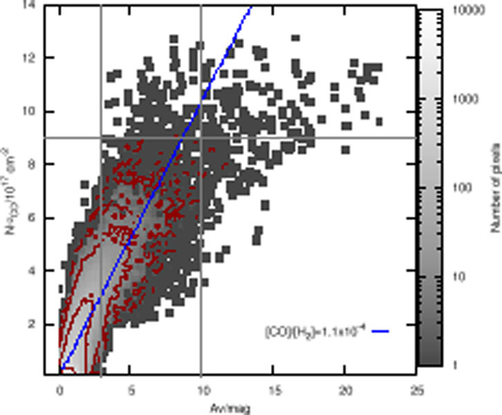Figure 3. Relation between CO column density and extinction in the Taurus molecular cloud (Pineda et al. 2010). The figure shows the pixel-by-pixel relation between gas-phase CO column density (obtained from 13CO) and AV. The blue line illustrates the "average" linear relation for 3 AV 10, N(12CO) 1.01 × 1017 AV cm-2 (implying CO/H2 1.1 × 10-4 for the assumed isotopic ratio). The linearity is clearly broken for AV 10. Pineda et al. (2010) show that linearity is restored to high AV after applying a correction for CO freeze-out into dust grain mantles.

Pineda et al. (2010) extend the aforementioned Goldsmith et al. (2008) study of Taurus by characterizing the relation between reddening (from the Two Micron All Sky Survey, 2MASS) and CO column density (derived from ¹³CO) to measure X_CO,20 2.1. They find that the relation between A_V and CO flattens for A_V 10 (Fig. 3), a fact that they attribute to freeze-out of CO onto dust grains causing the formation of CO and CO₂ ice mantles. Including a correction for this effect results in a linear relation to A_V 23. For A_V 3 the column density of CO falls below the linear relationship, likely due to the effects of photodissociation and chemical fractionation. Along similar lines, Heiderman et al. (2010) find that in Ophiuchus and Perseus CO can underpredict H₂ with respect to A_V for _mol > 200 M pc^-2 by as much as ~ 30%.

Paradis et al. (2012) recently used a high-latitude extinction map derived from 2MASS data using an extension of the NICER methodology (Dobashi et al. 2008, 2009) to derive X_CO in sample of nearby clouds with |b| > 10°. They find X_CO,20 1.67 ± 0.08 with a somewhat higher value X_CO,20 2.28 ± 0.11 for the inner Galaxy region where |l| < 70°. They report an excess in extinction over the linear correlation between total gas and A_V at 0.2 A_V 1.5, suggestive of a gas phase that is not well traced by either 21 cm or CO emission. We will return to this in Section 4.2.4.

4.2.3. Dust Emission

The use of extinction mapping to study N(H₂) is mostly limited to nearby Galactic clouds, since it needs a background stellar distribution, minimal foreground confusion, and the ability to resolve individual stars to determine their reddening. Most interestingly, the far-infrared emission from dust can also be employed to map the gas distribution. Indeed, dust is an extraordinarily egalitarian acceptor of UV and optical photons, indiscriminately processing them and reemitting in the far-infrared. In principle, the dust spectral energy distribution can be modeled to obtain its optical depth, _d(), which should be proportional to the total gas column density under the assumption of approximately constant dust emissivity per gas nucleon, fundamentally the product of the gas-to-dust ratio and dust optical properties.

How valid is this assumption? An analysis of the correlation between _d and HI was carried out at high Galactic latitudes by Boulanger et al. (1996), who found a typical dust emissivity per H nucleon of

(22)

with = 2, in excellent accord with the recent value for high latitude gas derived using Planck observations (Planck Collaboration et al. 2011c, who prefer = 1.8). They also identified a break in the correlation for N(HI) 5 × 10²⁰ cm^-2 suggestive of an increasingly important contribution from H₂ to N_H, in agreement with results from Copernicus (Savage et al. 1977). There is evidence that the coefficient in Eq. 22 changes in molecular gas. It may increase by factors of 2-3 at very high column densities (Schnee et al. 2008, Flagey et al. 2009, Planck Collaboration et al. 2011d), likely due to grain growth or perhaps solid state effects at low temperatures (e.g., Mény et al. 2007). Note, however, that recent work using Planck in the Galactic plane finds