


2.1. Heating and cooling of the starforming ISM in galaxies
At high redshift, the ionized ISM can be studied through a combination of optical emission lines (e.g. Lyα, Hα) and far–infrared (FIR) atomic fine structure lines (e.g. [C II], [N II], [O III]). The neutral medium can be studied with FIR atomic fine structure lines (e.g. [O I], [C I], [C II]). Unfortunately, HI 21cm emission from galaxies cannot be studied at redshifts z > 0.5 due to limited sensitivity, and must await the full square kilometer array (Carilli & Rawlings 2004). The atomic phase in high redshift systems can also be studied through absorption measurements through individual lines–of–sights (Wolfe et al. 2005).
In the molecular medium, the high gas densities protect molecules against UV photodissociation, because of the shielding by dust and self–shielding of H2 (Tielens 2005, Lequeux 2005, Dyson & Williams 1980). The molecular gas phase is thought to immediately preceed star formation (e.g. Leroy et al. 2008, Schruba et al. 2011) and this phase is thus most relevant to study a galaxy's potential to form new stars. The other phases of the ISM cannot form stars directly (but see, e.g., Glover & Clark 2012), unless they cool sufficiently to form cold and dense molecular gas. The processes in the ISM are highly dynamic, with new gas being accreted (e.g. through mergers or cold mode accretion, CMA, Sec. 5.1.2) and gas being lost through both stellar and black hole feedback processes (Sec. 4.7).
The temperature and density of the ISM is a result of environment, and is determined by a balance of heating and cooling. There are several mechanisms that lead to the heating of the molecular gas (e.g. Goldsmith 1978). Deep within dark molecular clouds, the main heating source is through cosmic rays (i.e. protons and electrons accelerated to GeV energies). Cosmic rays ionize H2 molecules, and the free electrons then transfer excess kinetic energy to other H2 molecules.
In molecular clouds associated with active star formation, UV heating is also invoked to explain molecular gas heating. In this picture, O and B stars that dominate the radiation in starforming regions (mostly in the far-UV, 6.0 eV < E < 13.6 eV, recall that 1 eV ∼ 104 K (1 eV = 11605 K)), turn their interface with the molecular clouds into photon dominated regions (PDRs; also historically known as photo–dissociation regions; Hollenbach and Tielens 1999). On the very surface, the CO is dissociated by UV radiation, and the dominant emission comes from atomic fine structure lines and H2 rovibrational lines, as well as dust continuum and PAH emission. Further into the region, dust–shielding and self–shielding allows for the persistence of CO, with the gas heated mainly by electrons that are released from the surfaces of dust grains due to UV absorption.
Related to the UV heating in PDRs is the heating that occurs through X–ray emission (X–ray dominated region, or XDR) emerging from AGN and/or hot plasmas heated by SNe, where the harder input spectrum of the X–rays penetrates further into the molecular clouds than the UV radiation (e.g. Meijerink et al. 2006). Both PDR and XDR regions are discussed in Sec. 2.6.2. Mechanical shock models have also been invoked to explain the extreme excitation conditions in nuclear starburst or other dense regions (e.g. Flower & Pineau des Forets 2003, Kristensen et al. 2008, Meijerink et al. 2013; Stacey et al. 2010; Nikola et al. 2011).
In terms of gas cooling, atomic fine structure lines have long been noted as being the dominant coolant of interstellar gas in star forming galaxies (Spitzer 1978), in particular, in cooler regions where permitted lines of Hydrogen cannot be excited (< 104 K; Sec. 2.8). As forbidden transitions, the lines are typically optically thin, and hence avoid line trapping (resonant scattering) in high column density regions. A few lines have ionization potentials that are higher than hydrogen (13.6 eV) and are thus cooling lines of the ionized medium only (e.g. [N II], [O III]). Others have lower ionization potentials, and thus also trace the neutral ISM (e.g., [C II], [O I], [C I]). Up to a few percent of the FUV energy from star formation in galaxies can go to gas heating via photo–electrons, which is reradiated by fine structure lines, principally the [C II] 158µm line (and in some cases [O I]). The majority of the stellar radiation goes into dust heating that is balanced through FIR emission, or is radiated directly into the Universe, in roughly equal proportions (depending on geometry and dust content, e.g., Elbaz 2002).
2.2. Tracing molecular gas: observable frequencies
The molecular gas mass in galaxies is dominated by molecular hydrogen, H2. Given the lack of a permanent dipole moment, the lowest ro–vibrational transitions of H2 are both forbidden, and perhaps more importantly, have high excitation requirements (the first quadropole line lies 500 K above the ground, significantly higher than temperatures in giant molecular clouds). As a consequence, only a very small fraction of the cool molecular gas can be studied through H2 emission in the infrared. This is the reason that historically, emission from tracer molecules have been used to detect molecular gas in galaxies, and from which the total molecular gas mass is then deduced. The molecule of choice has traditionally been carbon monoxide, CO, since it is the most abundant molecule after H2, has low excitation requirements ( ∼ 5 K for first excited state, see Sec. 2.3), and is easily observed from the ground (3 mm band) in its ground transition.
In general, tracer molecules show quantized rotational states populated based on collisions and the radiation field. For a linear polar molecule of moment of inertia, I, the orbital angular momentum is given by (Townes & Schalow 1975) L = nℏ and the corresponding rotational energy is Erot = L2 / 2I = n2 ℏ2 / 2I = [J(J + 1)ℏ2] / 2I with ΔJ = ±1 (conservation of angular momentum). The energy released from level J to J – 1 is: Δ Erot = [J(J + 1) − (J − 1) J] ℏ2 / 2I = ℏ2 J / I = h νline.
In reality this approximation is not strictly valid, as centrifugal forces will increase with J so that the bond (distance between atoms) will stretch, which in turn changes I. This effect leads to frequencies that are slightly lower than the first harmonic, eg. for CO, the line–spreading via rotational stretching of higher order transitions is of order 10 MHz to 15 MHz, or effectively 20 to 30 km s−1, allowing for unique redshift determinations based on just two transitions (e.g., Weiß et al. 2009). Depending on molecule, there can be other additional fine and hyperfine structures overlaid (i.e., magnetic and electrostatic interactions within the molecule; e.g., Riechers et al. 2007a for the case of CN).
2.3. Gas Temperatures & Critical Density
The kinetic temperature of the H2 molecules, Tkin is determined by the velocity distribution of the molecules following the Maxwell–Boltzmann distribution. The excitation of other tracer molecules, such as CO, is mostly determined by the number of collisions with H2 molecules as they are very abundant, massive and have a high cross section. It is often assumed that this kinetic gas temperature equals the temperature of the dust Tdust at high densities. However it should be noted that the heating and cooling processes of the dust and molecular gas phases are quite different and therefore thermal balance is not required.
Typically, rotational transitions are expressed as a function of critical density, ncrit, ie. the density at which collisional excitation balances spontaneous radiative deexcitation: ncrit = A / γ where A is the Einstein coefficient for spontaneous emission, A ∝ µ2 × ν3 in units of s−1, γ is the collision rate coefficient in units of cm3 s−1, and µ is the dipole moment of the molecular transition under consideration in the J = 1 state.
The Einstein coefficient A (see Tab. 1) is determined entirely by the physical properties of the molecule and is proportional to the frequency cubed (i.e. higher–J transitions have higher deexcitation rates). The collision rate coefficient γ however depends on the temperature of the gas (γ = < σ × v > where σ is the collision cross section and v is the velocity of the particle). Collision rate coefficients for the excitation of CO by H2 are given by Flower et al. (1985) and Yang et al. (2010), and are typically ∼ 3 to 10 × 10−11 cm3 s−1 for the low–J transitions and temperatures of 40–100 K.
| species | trans. | E.P. | λ | ν | Einstein A | ncrit |
| K | µm | GHz | s−1 | cm−3 | ||
| [O I] | 3P1 → 3P2 | 228 | 63.18 | 4744.8 | 9.0 × 10⁻⁵ | 4.7 × 10⁵ |
| 3P0 → 3P1 | 329 | 145.53 | 2060.1 | 1.7 × 10⁻⁵ | 9.4 × 10⁴ | |
| [O III] | 3P2 → 3P1 | 440 | 51.82 | 5785.9 | 9.8 × 10⁻⁵ | 3.6 × 10³ [⋆] |
| 3P1 → 3P0 | 163 | 88.36 | 3393.0 | 2.6 × 10⁻⁵ | 510 [⋆] | |
| [C II] | 3P3/2 → 3P1/2 | 91 | 157.74 | 1900.5 | 2.1 × 10⁻⁶ | 2.8 × 10³ |
| 50 [⋆] | ||||||
| [N II] | 3P1 → 3P2 | 188 | 121.90 | 2459.4 | 7.5 × 10⁻⁶ | 310 [⋆] |
| 3P1 → 3P0 | 70 | 205.18 | 1461.1 | 2.1 × 10⁻⁶ | 48 [⋆] | |
| [C I] | 3P2 → 3P1 | 63 | 370.42 | 809.34 | 2.7 × 10⁻⁷ | 1.2 × 10³ |
| 3P1 → 3P0 | 24 | 609.14 | 492.16 | 7.9 × 10⁻⁸ | 470 | |
| CO | J=1–0 | 5.5 | 2601 | 115.27 | 7.2 × 10⁻⁸ | 2.1 × 10³ |
| J=2–1 | 16.6 | 1300 | 230.54 | 6.9 × 10⁻⁷ | 1.1 × 10⁴ | |
| J=3–2 | 33.2 | 867 | 345.80 | 2.5 × 10⁻⁶ | 3.6 × 10⁴ | |
| J=4–3 | 55.3 | 650.3 | 461.04 | 6.1 × 10⁻⁶ | 8.7 × 10⁴ | |
| J=5–4 | 83.0 | 520.2 | 576.27 | 1.2 × 10⁻⁵ | 1.7 × 10⁵ | |
| J=6–5 | 116.2 | 433.6 | 691.47 | 2.1 × 10⁻⁵ | 2.9 × 10⁵ | |
| J=7–6 | 154.9 | 371.7 | 806.65 | 3.4 × 10⁻⁵ | 4.5 × 10⁵ | |
| J=8–7 | 199.1 | 325.2 | 921.80 | 5.1 × 10⁻⁵ | 6.4 × 10⁵ | |
| J=9–8 | 248.9 | 289.1 | 1036.9 | 7.3 × 10⁻⁵ | 8.7 × 10⁵ | |
| J=10–9 | 304.2 | 260.2 | 1152.0 | 1.0 × 10⁻⁴ | 1.1 × 10⁶ | |
| HCN | J=1–0 | 4.25 | 3383 | 88.63 | 2.4 × 10−05 | 2.6 × 10⁶ |
| J=2–1 | 12.76 | 1691 | 177.26 | 2.3 × 10−04 | 1.8 × 10⁷ | |
| J=3–2 | 25.52 | 1128 | 265.89 | 8.4 × 10−04 | 6.8 × 10⁷ | |
| J=4–3 | 42.53 | 845.7 | 354.51 | 2.1 × 10−03 | 1.8 × 10⁸ | |
| J=5–4 | 63.80 | 676.5 | 443.12 | 4.1 × 10−03 | 3.8 × 10⁸ | |
| J=6–5 | 89.32 | 563.8 | 531.72 | 7.2 × 10−03 | 7.1 × 10⁸ | |
| J=7–6 | 119.09 | 483.3 | 620.30 | 1.2 × 10−02 | 1.2 × 10⁹ | |
| J=8–7 | 153.11 | 422.9 | 708.88 | 1.7 × 10−02 | 1.8 × 10⁹ | |
| J=9–8 | 191.38 | 375.9 | 797.43 | 2.5 × 10−02 | 2.5 × 10⁹ | |
| J=10–9 | 233.90 | 338.4 | 885.97 | 3.4 × 10−02 | 3.3 × 10⁹ | |
Stars are created in cores of molecular clouds that have much higher densities than the bulk of the gas traced by CO(1–0). This is the reason why molecules with significantly higher dipole moments (leading to a higher A coefficient as A∝ µ2 and thus higher critical density) are typically observed. Typical dense gas tracers and their dipole moments are: CS: 1.958 D [Debye], HCO+: 3.93 D, HCN: 2.985 D, for comparison CO has a dipole moment of 0.110 D (Schöier et al. 2005). The downside of choosing these high density tracer molecules is their low abundance and resulting faint line fluxes (as discussed in Sec. 4.4).
As an example, Tab. 1 summarizes the Einstein coefficients for the different transitions of CO and HCN. The critical density for these molecules is given in the last column of the table. It is obvious that higher–J transitions need increasingly high critical densities to be visible. Einstein coefficients and collision rates for other molecules can be found in Schöier et al. (2005).
2.4. Brightness Temperature and line luminosities
Historically, radio astronomers express the surface brightness of a source as a Rayleigh–Jeans (RJ) brightness temperature for a blackbody at given temperature through Planck's law. Measurements of brightness temperature and surface brightness are thus equivalent measurements. Rather than expressing the temperature in terms of the Planck temperature, radio astronomers have traditionally used the low frequency (Rayleigh-Jeans) limit (kT / h ν≫ 1):
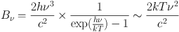 |
In this limit: TBobs = c2 / [2kνobs2] Iν, where Iν is the surface brightness. The RJ approximation is valid at centimeter wavelengths. However in the millimeter and particular submillimeter regime kT / hν = 0.7[λ / 1 mm][T / 10 K], the RJ approximation is no longer valid in many regions of astrophysical interest, and RJ brightness temperatures can no longer can be interpreted as a physical temperature. If one is interested in true temperatures, full Planck temperatures should be derived instead.
At high redshift, there are two commonly used ways to express line luminosities. One, Lline is expressed as the source luminosity in L⊙ or other rational units. The second, L′line, is expressed via the (areal) integrated source brightness temperature, in units of K km s−1 pc2. The following equations can be used to derive these two luminosities (Solomon et al. 1992):
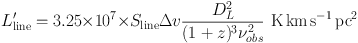 |
 |
where Sline Δ v is the measured flux of the line in Jy km s−1, DL is the luminosity distance in Mpc, and νobs is the observed frequency. Solving for S Δ v and equating leads to: Lline = 3 × 10⁻¹¹ νr3 L′line where νr is the rest frequency of the line. Note that L′line is directly proportional to the surface brightness TB, i.e. the L′line ratio of two lines give the ratio of their intrisic, source–average surface brightness temperatures TB. If the molecular gas emission were to come from thermalized, optically thick regions, L′line is constant for all J levels.
The question often arises which quantity to quote in a paper, Lline or L′line? Both have their justification: e.g. if one is interested in comparing the power that is being emitted through a given line to calculate the cooling capability (e.g. in relation to the FIR luminosity, Lline / LFIR) one uses the Lline definition. The L′line is commonly used to translate measured CO luminosities to H2 masses using the conversion factor α. Also, for thermalized molecular gas emission L′line is approximately constant for all transitions. It is good advice to give both quantities in a paper, but in all cases also the measured integrated fluxes of the lines Sline Δ v (in units of Jy km s−1).
2.5. CO luminosity to total molecular gas mass conversion factor
The conversion factor relating CO(1–0) luminosity to total molecular gas mass (dominated by H2) in the nearby Universe has been reviewed recently by Bolatto et al. (2013). We briefly summarize the main points in this section.
Molecular gas in the Milky Way and nearby galaxies is predominantly in giant molecular clouds with overall sizes up to 50 pc. Hence, early work on the conversion factor focused on GMCs. In nearby systems (including the Milky Way) the clouds can typically be spatially resolved, and hence the conversion factor considered, XCO, is the ratio of column density (H2 molecules per cm2) to CO velocity integrated surface brightness (K km s−1), while for distant galaxies spatially integrated quantities are usually measured, and the conversion factor αCO is then the ratio of total mass (in M⊙) to total CO line luminosity (K km s−1 pc2). The ratio, X / α = 4.6 × 10¹⁰ pc2 cm−2 M⊙−1 = the number of hydrogen molecules per solar mass, converted to the appropriate units and corrected by a factor 1.36 for Helium.
Numerous techniques have been used to determine the conversion factor in GMCs, including: (i) a comparison of CO columns derived from isotopic measurements to H2 columns derived from optical extinction measurements using a standard dust–to–gas ratio (Dickman 1978, 1975; Dame et al. 2001), (ii) a comparison of γ–ray emission to CO surface brightness, where the γ–rays result from the interaction between cosmic rays with H2 molecules (Strong & Mattox 1996, Bloemen 1989, Hunter et al 1997), and (iii) modeling GMCs as self–gravitating clouds. In the latter case, a key discovery was the correlation between line width and cloud size, with line width increasing as the square root of cloud size (the ‘Larson relations'; Larson 1981). This functional form implies a constant surface density ∼ 100 M⊙ pc−2 for GMCs (Solomon et al. 1987), and that the CO luminosity is linearly proportional to cloud virial mass. Indeed, this relationship provides the theoretical under–pinning of the use of CO luminosity to derive total gas mass in the case of optically thick emission (Solomon et al. 1987; Dickman et al. 1986), where luminosity is dictated principally by line width. Bolatto et al. (2013) summarize these results, and conclude that a value of XCO = 2 × 10²⁰ H2 molecules per cm−2 /(K km s−1), or αCO ∼ 4 M⊙ / (K km s−1 pc2), is appropriate for GMCs in the MW and nearby spiral galaxies, with a factor two (0.3 dex) scatter.
Draine et al. (2007) hypothesized that, if the abundance of the elements can be assumed to be proportional to the Oxygen abundance, and adopting a Milky–Way fraction of elements tied up in grains, then Mdust / Mgas = 0.010 [(O/H)] / [(O/H)MW]. Using observations of nearby galaxies, they showed that the gas columns derived from the IR thermal dust emission are consistent with XCO = 4 × 1020 cm−2 / (K km s−1 and metallicities between 0.3 and 1 solar for their galaxy sample. Leroy et al. (2011) use an empirical dust–to–gas ratio approach in nearby galaxies and obtain similar results, showing that the lowest metallicity galaxies clearly have much higher conversion factors. They suggest that decreased dust shielding in low metallicity environments leads to CO–free, but still H2 rich, cloud envelopes (see also Schruba et al. 2012; Sandstrom et al. 2013).
A different picture has emerged for nearby nuclear starburst galaxies, including the nuclei of dwarf starbursts like M 82 and NGC 253, corresponding to Luminous Infrared Galaxies, or LIRGs (LIR ∼ 1011 L⊙), and ultraluminous infrared galaxies (ULIRGs) such as Arp 220 (LIR ∼ 1012 L⊙). It was noted early–on that a Milky Way conversion factor leads to a molecular gas mass larger than the dynamical mass in some of these systems (Bryant et al. 1999). In their seminal analysis of CO radiative transfer and gas dynamics in starburst nuclei of ULIRG on scales < 1 kpc, Downes & Solomon (1998) find a characteristic value of αCO ∼ 0.8 M⊙ / (K km s−1 pc2) in these systems. The lower value of α implies more CO emission per unit molecular gas mass. They hypothesize that much of the CO emission is not from virialized GMCs, but from an overall warm, pervasive molecular inter–cloud medium. In this case the linewidth, and hence line luminosity (for optically thick emission), is determined by the total dynamical mass (gas and stars), as well as ISM pressure. Narayanan et al. (2012) show that the lower α value in starbursts is due to warm gas that is heated by dust (at densities > 104, such energy exchange is efficient), as well as large, non-virial line widths from the GMCs. More recently, Papadopoulos et al. (2012) suggest that the molecular gas heating processes in nuclear starbursts may be very different than is typically assumed for PDRs, with cosmic rays and turbulence dominating over photons.
In general, the value of α is likely a function of local ISM conditions, including pressure, gas dynamics, and metallicity, and remains an active area of research for nearby galaxies (Ostriker & Shetty 2011; Narayanan et al. 2012; Narayanan & Hopkin 2012; Papadopoulos et al. 2012, Leroy et al. 2013, Schruba et al. 2012, Sandstrom et al. 2013). We note that the conversion factor has been calibrated using observations of CO(1–0) in nearby galaxies. These low order transitions redshift to centimeter wavelengths at z > 2.
2.6. Modeling the line excitation
Many observations of galaxies at high–redshift are unresolved, and studies of the global CO excitation play an important role in constraining their average molecular gas properties. This CO excitation, i.e. the relative strengths of the observed rotational transitions, is sometimes referred to ‘CO spectral line energy distributions', ‘CO SLEDs' or ‘CO excitation ladder'. We here use the term ‘CO ladder', as the measured quantity is the emission of a given rotational transition J. We note that some authors also chose to plot spectral power distributions (i.e. plotting L instead of Sν × dV as a function of rotational number J).
The excitation temperature determines the population of the molecular levels through the Boltzmann distribution. Under the assumption of local thermodynamical equlibrium (LTE) this excitation temperature will be equal to the kinetic temperature of the gas. ‘Thermal' excitation means that the population of all levels is according to the Boltzmann distribution. The excitation is ‘sub–thermal' if the population of the high levels is less than that given the kinetic temperature of the gas, as occurs in lower density environments where collisional excitation cannot balance spontaneous emission rates. We briefly discuss the commonly used techniques to model the excitation of the various levels of molecular line emission.
2.6.1. Escape propability/LVG models. One basic tool commonly used to model the excitation of the molecular gas emission is the large velocity gradient (LVG) method (e.g. Young & Scoville 1991). In the following we will discuss this model for the CO molecule, but the same modeling can be done for any molecule. The model calculates for a given temperature Tkin, H2 density, CO abundance ([CO] / [H2]), and velocity gradient dv/dr, how the various levels of the CO are populated through collisional excitation with H2. Some models and their dependence on temperature and density are illustrated in Fig. 3 (see also Figures in van der Tak et al. 2007). Since the CO emission is optically thick (at least in the low–J transitions) the emission would have difficulties escaping the cloud, which is why a velocity gradient is introduced in the model that describes how many photons can eventually leave the cloud. The justification for implementing such a gradient is that in reality the molecular medium is turbulent which enables CO photons to escape their parental clouds. The LVG codes also take the redshift of the source into account which dictates the temperature of the cosmic microwave background (CMB, Sec. 2.10). Once the occupation numbers of the different levels are calculated, the optical depths τ for the transitions as well as the Rayleigh–Jeans brightness temperatures TB (which would be constant in LTE) and the resulting line intensities are derived.
In this way, for a given set of parameters, the expected line intensities for any molecule can be derived (assuming certain abundances of the molecule under consideration). In principle, the measurement of the line emission ladder of a number of different molecules thus puts tight constraints on the temperture and density of the gas. This assumes that these lines probe the same volume, which may not hold for those molecules tracing very high densities (e.g. HCO+ and HCN). Of particular interest is adding different isotopomers, such as 13CO or C18O as these are more optically thin than the 12C16O emission, and are thought to originate from the same volume as 12C16O, at least on GMC scales.
2.6.2. PDR and XDR models In PDR (Photo–dominated regions) and XDR (X–ray dominated regions) models a cloud is exposed to a radiation field from which the temperature and density distribution of the H2 molecules is derived. With the resulting values for Tex and density a code similar to LVG is then run to calculate the line intensities of the rotational transitions of the molecules under consideration. A difference with respect to the LVG models is that abundances of species are calculated based on the radiation field and the gas column density. The main difference between the PDR and XDR codes is that PDRs only exist at the surface of clouds (where they emit fine structure lines of [C I], [C II] and [O I], and rotational lines of CO in the submillimeter). In the XDR phase (further inside the cloud) the [O I], [C II], and [S III] lines are main coolants in the sub–millimeter regime (Meijerink & Spaans 2005). One limitation of most PDR / XDR models is that they are based on (one–dimensional) infinite slabs – i.e. they do not have a confined volume. As a consequence no mass estimates are typically given by the codes. The gas temperatures calculated in PDR/XDR models are still quite uncertain and depend on the code used, especially in the high–denisty, high–UV case (e.g., Röllig et al. 2007). Given the high excitation measured in nearby galaxies based on Herschel data (up to J ∼ 30, Hailey–Dunsheath et al. 2012), shock heating is also invoked to explain extreme CO excitation (see also Meijerink et al. 2013).
One complication in all the models above is that it is now established that the high–J rotational transitions of some molecules, e.g. HCN, are not only excited through collisions (as the critical densities of some of the detected high–J lines are extremely high, ∼ 109 cm−3, i.e. they are not even being reached in the cores of GMCs). One potential mechanism to excite the observed high–J HCN rotational modes is through the infrared stretching and bending modes of HCN at 3, 5 and 14 microns (this is referred to as ‘infrared pumping' of the rotational levels, e.g. Weiß et al. 2007a). Similar pumping may be in place even in the case of CO emission and may explain the very high–J excitation seen in some local galaxies (above references, and Harris et al. 1991 for radiative trapping leading to enhanced mid–J CO emission).
Water is thought to be one of the most abundant molecules in galaxies, present predominantly in icy mantels of dust grains in cold environments (Tielens et al. 1991; Hollenbach et al. 2008). In warmer environments, water in the gas phase is thought to play an important role in cooling (Neufeld & Kaufmann 1993, Neufeld et al. 1995). The rotational transitions of water have high Einstein A values, and thus very high critical densities (> 108 cm−3), i.e. collisional excitiation can only happen in the very centres of dense cloud cores and other excitation mechanisms, in particular infrared pumping, are typically invoked.
Naturally, water lines at low redshift are very difficult to observe from the ground given the Earth's atmosphere. Herschel Space Observatory observations enabled the first detections of submillimeter lines of H2O in nearby galaxies, other than Masers (Mrk 231: Van der Werf et al. 2010, Gonzales–Alfonso et al. 2010, M 82: Weiß et al. 2010) These observations have yielded very different results between the objects: Mrk 231 revealed a rich spectrum of H2O lines but the ground–state lines remained undetected (Van der Werf et al. 2010). In M 82 no highly excited emission was found (Panuzzo et al. 2010) but many low–excitation lines (Weiß et al. 2010). Generally speaking, the water emission line spectrum is very complex and not straightforward to interpret if only one or a few lines are measured (Gonzalez–Alfonso et al. 2010). We discuss recent high–redshift detections of water lines in Sec. 4.4.
2.8. Atomic Fine Structure lines
The atomic fine structure lines (FSLs) are major coolants of cooler interstellar gas (Section 2.1). Table 1 summarizes key parameters of important sub–millimeter atomic fine structure lines.
2.8.1. Singly Ionized Carbon: [C II] is the strongest line from star forming galaxies at radio through FIR wavelengths (eg. [C II] line fluxes are typically > 103 times stronger than CO(1–0) in star forming galaxies), and in particular, [C II] 158µm is the strongest line from the cooler gas in galaxies (< 104 K).
The ratio of [C II] / FIR luminosity for the Milky Way is 0.003, and this value holds in nearby disk galaxies, with a relatively large scatter (factor three; e.g. Malhotra et al. 1997, 2001). However, the ratio appears to drop significantly at FIR luminosities above 1011 L⊙. One explanation for this drop is a reduction in the heating efficiency by photoeletric emission from dust grains in high radiation environments due to highly charged grains. This explanation is supported by the fact that the [C II] / FIR ratio is also a decreasing function of increasing dust temperature (e.g., Malhotra et al. 2001, Luhman et al. 2003). High dust opacity/absorption at 158µm may also decrease the [C II] / FIR ratio in high luminosity systems.
[C II] has a lower ionization potential than H I (11.3 eV vs. 13.6 eV), hence [C II] traces both the cold neutral medium (CNM) and ionized gas. This makes [C II] less easy to interpret, in particular if the emission cannot be resolved spatially. The [C II] luminosity is not a simple function of star formation rate, nor is there a simple dependence between [C II] luminosity and the total mass of the ISM. In an early study, Stacey et al. (1991) argue that roughly 70% of the total [C II] emission from nearby spiral galaxies comes from PDRs, and recent Herschel observations shows a possible correlation between the [C II] luminosity and the 11.3µm PAH feature, suggesting a close correlation between PDRs and [C II] emission (Sargsyan et al. 2012). Herschel imaging has also shown significant differences in the spatial distribution of the [C II] emission and CO emission on scales ≤ 300 pc in nearby galaxies (Mookerjea et al. 2011; Rodrigues-Fernandez et al. 2006) (see also Cormier et al. 2010).
A clear trend for increasing [C II] / FIR ratio with decreasing metallicity has been established (Cormier et al. 2010; Israel & Mahoney 2011). Lower metallicity leads to lower dust and higher UV mean free paths. The decreased dust–shielding in PDR regions leads to deeper photo–dissociation into the molecular clouds and increased photo–electric heating efficiencies leading to higher [C II] luminosities relative to the FIR. High–redshift observations of [C II] are discussed in Sec. 4.3.2.
2.8.2. Atomic Carbon: [CI] Because the 3P fine–structure system of atomic carbon forms a simple three–level system, detection of both optically thin carbon lines, C I (3P1 → 3P0) and C I (3P2 → 3P1) enables one to derive the excitation temperature, neutral carbon column density and mass, independent of any other information (e.g., Ojha et al. 2001, Weiß et al. 2003, Walter et al. 2011). A combination of this method (using [C I]) with the aforementioned CO excitation ladder is particularly powerful as it eliminates some of the degeneracy frequently found in CO radiative transfer models under the assumption that [CI] traces the same regions as CO (see discussion in Sec. 4.1).
Studies of atomic carbon in the local universe have been carried out in molecular clouds of the galactic disk, the galactic center, M 82 and other nearby galaxies (e.g., White et al. 1994; Stutzki et al. 1997; Gerin & Phillips 2000; Ojha et al. 2001; Israel & Baas 2002; Israel 2005). These studies have shown that [C I] is closely associated with the CO emission independent of environment. Since the critical density for the C I (3P1 → 3P0) and CO(1–0), lines are both ncr ≈ 103 cm−3, this suggests that the transitions arise from the same volume and share similar excitation temperatures (e.g. Ikeda et al. 2002). We discuss high–redshift detections of [C I] in Sec. 4.3.1.
2.8.3. Other fine structure lines: [N II], [O I], [O III]. Beyond [C II] and [C I], there are a number of other far–infrared fine structure lines that are potentially important physical diagnostics for the ISM, in particular the lines from [O I] 63 µm, [O III] 52 µm and 88 µm, and [N II] 122 µm and 205 µm. While typically 10 times weaker than [C II], the oxygen line strengths increase dramatically with the hardness of the radiation field, such that in AGN environments the [O III] 88 µm can be stronger than [C II] (Spinoglio et al. 2012; Spinoglio & Malkan 1992; Genzel & Cesarsky 2000, Stacey et al. 2010). Most of these lines are at even higher frequencies than [C II] and are thus difficult to observe even in the high–redshift universe.
The ionization potential of carbon, oxygen, and nitrogen are 11.3 eV, 13.6 and 14.5 eV, respectively. Hence, [C II] traces both the neutral and ionized medium, while oxygen and nitrogen trace the ionized medium only (except for [O I]). The [N II] 122 µm / [O III] 88 µm ratio is a sensitive measure of hardness of the radiation field since these two lines have similar critical densities for excitation ( ∼ 300 to 500 cm−3), but very different ionization potentials (35 eV for [O II]). [C II] 158 µm and [N II] 205 µm have essentially the same critical density for thermal excitation ( ∼ 45 cm−3), hence the ratio of [C II]158 / [N II]205 indicates the fraction of [C II] emission from ionized gas, assuming only a gas phase C/N abundance (Oberst et al. 2006, Walter et al. 2009a, Decarli et al. 2012, Ferkinhoff et al. 2010, 2011). In this case, the [C II]158 / [N II]205 ratio for ionized gas ranges between 3 and 4 (Fig. 2 in Oberst et al). Oberst et al. (2006) show that the [N II] 122 µm / [N II] 205 µm ratio is a densitometer, with a value of ∼ 0.5 for densities below 102 cm−3, rising to 10 for densities greater than 103 cm−3.
2.9. Relation to far–infrared emission and SFRs
In this review, we concentrate on the molecular gas properties of high redshift galaxies. To put the physical properties of the ISM into perspective, we will also use the far–infrared (FIR) emission and star formation rates in galaxies. For reference we here give the equations that are commonly used to derive IR/FIR luminosities and star formation rates from single–band FIR continuum measurements. We stress that the numbers that follow are appropriate for ‘dusty' SEDs typically found at high redshift, but that the relations will be a strong function of galaxy properties, such as the star formation activity and dust optical depth. The following equations are to first order independent of redshift for z > 1, given the inverse K–correction in the sub–millimeter regime (e.g. Blain 2002; Kennicutt & Evans 2012).
The IR luminosity LIR is defined from 8–1000 µm, whereas the FIR luminosity LFIR is commonly defined from 40–400 µm (Sanders et al. 2003). LIR is typically ∼ 30% higher than LFIR for ‘dusty' SEDs. Some authors also define FIR from 42–122 µm (Helou et al. 1985) – this latter definition gives LFIR that are 20–30% smaller that the LFIR definition above.
In measured flux densities at 250 GHz and 350 GHz (850 µm), the following relations are commonly used: LFIR[L⊙] ∼ 1.2 × 10¹² S350 GHz[mJy] (e.g. Genzel et al. 2010, Pope et al. 2006, Magnelli et al. 2010), LFIR[L⊙] ∼ 3 × 10¹² S250 GHz[mJy] (e.g. Bertoldi et al. 2003, Omont et al. 2001), with significant dependencies on the actual shape of the SED. As Scoville (2012) points out, a continuum measurement around 1 mm wavelengths (observed frame) is not suited to give good estimates of LIR given the unknown intrinsic dust SED, at least for redshifts z < 4. However, it gives a good estimate on the dust mass (given that the dust is optically thin, and that the dust temperatures are not found to vary greatly).
The SFR can be calculated from the IR luminosities following: SFR ∼ δMF × 1.0 × 10⁻¹⁰ LIR where δMF depends on the stellar population (this assumes that the galaxy is dusty i.e. that all of the power radiated by young stars is absorbed by dust and re–emitted in the infrared; also that there is no contribution of the AGN to the FIR emission). For a range of metallicities, starburst ages (< 100 Myr) and initial mass functions (IMFs) Omont et al. (2001) find: 0.8 < δMF < 2. Typically a δMF = 1.8 is appropriate for a Salpeter IMF (e.g. Kennicutt 1998), and δMF ∼ 1.0 for a Chabrier IMF.
We adopted FIR luminosities for all high–redshift sources in which line emission as been detected (Tab. 3). These FIR luminosities have been derived using various different methodologies and therefore should be treated with caution. Wherever available, we adopted the FIR luminosities given by indivdual studies but caution that not all authors have adopted the same ‘FIR' definition. E.g. LFIR is frequently adopted to go from 8–1000 µm, whereas strictly speaking this is the definition of the IR luminosity (see above). For the purpose of this review we simply set LFIR ∼ LIR. For each source in the table we have computed the FIR luminosities as follows: 1) if a LFIR value is already reported in the literature (e.g., based on dust SED fitting of multiple photometric information) we use the most up-to-date estimate available; 2) for a number of color–selected galaxies, only an estimate of the SFR is available. In this case, we convert it into dust luminosity using the relation log LFIR = log SFR − log(1.3) + 10, where LFIR is in solar units and SFR is in solar masses per year (see Genzel et al., 2010). 3) If only a continuum estimate is available, we use the 850 µm flux to infer continuum luminosity, assuming the Arp 220 template by Silva et al. (1998) and integrating from 8 µm – 1000 µm. To first order, log LFIR ≈ log(1.2 × Fν(850 µm)) + 12, where Fν(850 µm) is the flux density at 850 µm, expressed in mJy. If 850 µm measurements are not available, we use the 1200 µm measurement instead (in this case, log LFIR ≈ log(Fν(1200 µm)) + 12.36)).
The temperature of the CMB at redshift z is given by: TCMB(z) = 2.73 × (1 + z). At a redshift of z = 6, TCMB = 19.1 K, meaning it is warmer than the dust temperature of Milky Way at present. As the dust will always be heated by photons of the CMB (through absorption), the minimum dust temperature will be that of the CMB (and the kinetic temperature of the gas will equal the thermal dust temperature at high enough densities, da Cunha et al. 2013). As brightness temperature measurements are by definition always done with respect to the background (i.e. the CMB) it will be increasingly difficult to detect cold dust emission at high redshift.
The molecular gas is affected in two ways by the CMB: First, the higher temperature of the CMB will lead to an increase of the line excitation, and thus the line luminosities (e.g., Obreschkow et al. 2009a, da Cunha et al. 2013). Second, the observing background against which the line is measured also increases. The relative effect of the CMB will depend on the intrinsic excitation temperature of the gas (Combes et al. 1999, Obreschkow et al. 2009a, da Cunha et al. 2013). For example, for molecular gas at a temperature much higher than the CMB, the relative decrease in line flux will be much lower than in a case where the molecular gas temperature is almost equal to the CMB. As a result of this, the shape of the observed CO ladder for a source with given temperature and density will also change as a function of redshift: The peak of the SED will shift to higher–J values as the lower–J transitions are most easily affected by the effects of the CMB (da Cunha et al. 2013). A suppressed measurement of the CO lines also implies that the conversion factor α will change as a function of CMB temperature.
It should be noted that all CO detections at very high redshift (z > 5), i.e. where TCMB is significant, are to date from galaxies that harbor hyper–star forming environments (e.g. the z ∼ 6 quasars and the few known SMGs at z > 5 have SFRs of ∼ 1000 M⊙ yr−1) with accompanying high temperatures of the ISM, ranging from 35–50 K, or at least a factor two warmer than the CMB. However it is clear that in lower temperature environments, more typical of lower luminosity star forming galaxies, the consequences of the CMB will be significant: the lowest–J lines will be faint at z > 4, and other cool ISM tracers may be required, such as [C II].