


PROFILE FITTING - ALLSTAR
Now that we have that dreadful discussion out of the way, we come to the heart of crowded-field photometry - the actual fitting of the model stellar profile to star images. I've already explained the basic principle several times. You simply use non-linear least squares to fit the model profile to the actual data, to determine four unknowns per star: the x0, y0 position of the star's centroid, the star's brightness, and the local sky brightness (6). If two stars are blended together, then you solve simultaneously for seven unknowns: two x0's, two y0's, two C's, and one B. If three stars are blended, you solve for ten unknowns, and so on.
To work this method up into a practical computer program, however, there are some details to consider. The first of these is you must decide exactly which pixels to use in the fits for any given star. In the examples of two-dimensional profile fits that I showed you two days ago, I fit the model profile to all pixels contained within a large rectangular area around the star. This is not really a very practical definition of the "fitting region" in a crowded field. Say you have a frame where the stellar images have a full-width at half-maximum of 3 pixels. A bright star in such a frame might have a profile which could be traced out to a radial distance of 12 pixels. If you were to use a rectangular box including the entire stellar profile, it would have sides of ± 12 = 25 (think about it) pixels and would contain 625 pixels. This is a lot of data for one little star. Worse, a rather crowded frame, in my experience, could contain as much as one star per every 30 - 50 pixels (a 300 x 500 frame with critical sampling, if it is crowded, can contain 3,000 - 5,000 stars that are worth trying to reduce). The "fitting region" around the star of interest, then, may be expected to contain ~ 20 other stars: if you try to reduce simultaneously all stars that are blended - in the sense that their fitting regions contain some pixels in common - you'll surely be reducing every star in the frame all at once, and you'll be trying to invert 15,000 x 15,000 matrices. Forget it.
Instead, you must adopt much smaller fitting regions around each
star. In the sorts of
frames I was talking about earlier, with FWHM ~ 3 pixels (HWHM ~ 1.5
pixels), I've been
using circular fitting regions with radii of order 2.5 - 3 pixels. (Why
do some programs use
a rectangular fitting region? Sure, it's a bit easier to program, but
stars are round, and
why should a pixel which is  2
. 3 pixels from the star's centroid in a
diagonal direction be
included in its solution, while one which is the same distance away to
the right or left or
above or below is excluded?) In the simultaneous reductions of every
star in a CCD frame,
ALLSTAR starts with the initial guesses for all the unknown parameter
values (x0, y0, and
C for every star in the frame), subtracts the model profiles implied by
these values from
the image and, using the residuals from these subtractions, does a
single nonlinear-least-squares
iteration for every star in the frame. For each individual star, ALLSTAR
considers
only the residuals in the 2.5 - 3-pixel circular fitting region if the
star is isolated. However,
any stars whose fitting regions overlap are included in the same matrix
inversion for this
iteration. Then, after a single correction has been derived for each of
the parameters of
every stars in the frame, the entire profiles implied by the new values
of x0, y0, and C - out
to the full radius to which the PSF has been defined - are subtracted
from the frame,
and another iteration is performed on every star in the image based upon
the new set of
residuals. When any individual star seems to have fully converged to its
"best" parameter
values, these values are written to a disk file, the star is subtracted
permanently from the
image, and subsequent iterations continue with whatever stars are
left. As more and more
stars converge and are removed from the problem, the iterations progress
faster and faster. It gets quite exciting toward the end.
2
. 3 pixels from the star's centroid in a
diagonal direction be
included in its solution, while one which is the same distance away to
the right or left or
above or below is excluded?) In the simultaneous reductions of every
star in a CCD frame,
ALLSTAR starts with the initial guesses for all the unknown parameter
values (x0, y0, and
C for every star in the frame), subtracts the model profiles implied by
these values from
the image and, using the residuals from these subtractions, does a
single nonlinear-least-squares
iteration for every star in the frame. For each individual star, ALLSTAR
considers
only the residuals in the 2.5 - 3-pixel circular fitting region if the
star is isolated. However,
any stars whose fitting regions overlap are included in the same matrix
inversion for this
iteration. Then, after a single correction has been derived for each of
the parameters of
every stars in the frame, the entire profiles implied by the new values
of x0, y0, and C - out
to the full radius to which the PSF has been defined - are subtracted
from the frame,
and another iteration is performed on every star in the image based upon
the new set of
residuals. When any individual star seems to have fully converged to its
"best" parameter
values, these values are written to a disk file, the star is subtracted
permanently from the
image, and subsequent iterations continue with whatever stars are
left. As more and more
stars converge and are removed from the problem, the iterations progress
faster and faster. It gets quite exciting toward the end.
A tiny fitting region for each star is possible because, while the profile for a bright star can extend many HWHM's from the center, really most of the photometric and positional information is contained within a couple of HWHM's. A tiny fitting region is necessary, because otherwise the solutions become completely intractable if there are more than a couple hundred stars in the frame. However, such tiny fitting regions have their own problems. In particular, because the stellar profile has not, in general, gone to zero surface brightness by the time the edge of the fitting region has been reached, it is possible to get into paradoxical solutions. For instance, when some particular pixel is included in the fitting region for the star, the star's centroid may get corrected so as to shift that pixel out of the fitting region; then, without that pixel, the solution corrects the star's centroid so as to bring that pixel back into the fitting region. The solution could wobble back and forth forever. Alternatively, you might have a situation where including a particular pixel in the solution keeps the pixel in the fitting region, and excluding it keeps it out of the fitting region: two slightly different starting guesses could then come up with completely different final answers for the same star from the same data. For each of these two situations, there is no good way to determine which of the two possibilities is the "better" answer without including every pixel in the frame in the solution for every star in the frame. One practical answer is to increase the adopted radius of the fitting region slightly, and then to taper off the weights assigned to the pixels as the edge of the fitting region is approached, using some arbitrary radial weighting function like that illustrated in Fig 4-4. Then whatever pixel was causing the solution either to dither or to split into two distinct answers can achieve partial weight somewhere out near the edge of the fitting region, and the solution can happily converge to some balanced intermediate value. I confess that I can't demonstrate analytically that this intermediate solution is "better" than either of the two previous alternatives, but intuitively I suspect that it is. After all, partial weights for pixels straddling the edge of the fitting region is physically sensible: partial weights for pixels partially in the fitting region. The precise formula which one uses to compute those partial weights won't be very important. I can say on the basis of considerable experience that at least this method allows the solution to converge to some reasonable value, so you can finish reducing this frame and get on to the next one.

|
| Figure 4-4. |
You may have noticed that a couple of paragraphs back, I said nothing
about ALLSTAR
correcting the sky value associated with each star. Of course it could
do this - one would
merely solve for 3N + 1 unknowns (for a constant sky level,
3N +3 for a sloping plane, ...)
- but in general I don't. Because only a few pixels per star are
included in fits, and those
pixels are restricted to radii which are pretty much still well within
some star's profile, it is
not really practical - under the conditions I have described - to
redetermine the sky as
part of the least-squares fits. Instead, I usually assume that the sky
value determined during
the aperture photometry is correct, and use that. I think that this is
not necessarily a Bad
Thing. In the other method, where the stellar profile plus the sky value
are all determined
together by a least-squares fits to some large region, there may be at
most some hundreds of
pixels which can contribute meaningfully to the determination of the sky
value. In contrast,
for the sky annulus which is used to determine the sky value in the
aperture photometry, I typically set an inner radius
 20 pixels and an outer
radius ~ 35
pixels. This region thus
contains some
20 pixels and an outer
radius ~ 35
pixels. This region thus
contains some  .
(352 - 202) = 2600 pixels, as
compared to only a few hundred; on our
VAX 11/780 or a microVAX, the Kitt Peak algorithm can get a sky value
from these 2600
pixels in considerably less than a second, while a full-blown nonlinear
least-squares solution
to 625 pixels would take far longer than this. Furthermore, the
algorithm which the Kitt
Peak software uses is highly robust against contamination by other stars
or by defective
pixels, while a standard least-squares solution in the big rectangular
area would have to
be very careful to avoid being affected by such problems. A little
circular fitting region of
radius, say, 3 pixels would contain some 28 pixels in all, but because
of the tapered radial
weights, the effective area would be somewhat smaller - maybe 20
pixels. The probability
of contamination in this area is ~ 625/20 = 30 times smaller than in the
big area.
.
(352 - 202) = 2600 pixels, as
compared to only a few hundred; on our
VAX 11/780 or a microVAX, the Kitt Peak algorithm can get a sky value
from these 2600
pixels in considerably less than a second, while a full-blown nonlinear
least-squares solution
to 625 pixels would take far longer than this. Furthermore, the
algorithm which the Kitt
Peak software uses is highly robust against contamination by other stars
or by defective
pixels, while a standard least-squares solution in the big rectangular
area would have to
be very careful to avoid being affected by such problems. A little
circular fitting region of
radius, say, 3 pixels would contain some 28 pixels in all, but because
of the tapered radial
weights, the effective area would be somewhat smaller - maybe 20
pixels. The probability
of contamination in this area is ~ 625/20 = 30 times smaller than in the
big area.
|
| Figure 4-5. |
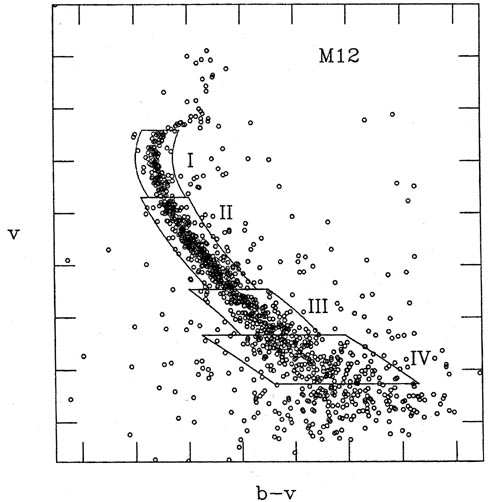
All of the handwaving arguments in the world won't convince you that it's OK not to determine the sky level as part of the least-squares profile fits (they didn't convince me, anyway), so I ran some tests. Figs. 4-5 and 4-6 show two instrumental color-magnitude diagrams; Fig. 4-5 is for the globular cluster M12, and Fig. 4-6 is for our old friend 47 Tucanae, with a little bit of the Small Magellanic Cloud in the background. Each of these color-magnitude diagrams is based on a single pair of frames. I repeated the reductions of these four images, using NSTAR (an earlier, slower, more primitive version of ALLSTAR), and seven sets of conditions: (1) adopting the sky-brightness value which PHOTOMETRY obtained for each star as correct, and using a radius for the fitting region of 2 pixels; (2) - (4) determining a constant sky-brightness value for each group of blended stars, with fitting radii of 2, 4, and 6 pixels; and (5) - (7) fitting a sloping plane to the sky underneath each group of blended stars, with fitting radii of 2, 4, and 6 pixels. Tables 4-1 and 4-2 show the results of these tests, in the form of the mean absolute half-width of the cluster sequence contained in each of the boxes in Figs. 4-5 and 4-6 (note that box IV in the 47 Tuc diagram is the upper main sequence of the SMC; the gap between boxes I and II in this figure is to exclude the red horizontal branch of the SMC, which lies on top of 47 Tuc's main sequence at this point). For the 47 Tuc reductions, I have also listed the execution time required to reduce the two images. As you can see, solving for the sky as part of the profile fits increases the scatter, typically by of order 18%, while increasing the typical execution time from 12.4 hours to 18.3 hours: in effect you are getting 28% less information while doing 46% more work.

|
| Figure 4-6. |
Of course, simply adopting the PHOTOMETRY values of the sky brightness is not
the best idea if the sky changes significantly on the scale of the sky
annulus. In 1988,
Bill Harris and I did a pretty extensive study of the globular cluster
M92. There, both
the cluster background and some scattered light from bright stars just
off the side of the
frame made for a spatially varying sky brightness. What we did was to
perform one set
of profile fits, employing the sky values from PHOTOMETRY. We then
subtracted all the
visible stars from the frame, and passed a median filter over the image:
for each pixel in the
subtracted image, we determined the median of all pixel values in a
circular region centered
on that pixel. Where a pixel was "missing," whether because it was "bad"
or because the
circular region extended beyond the edge of the frame, the diametrically
opposite pixel
was also omitted from the median. This properly preserves the brightness
gradients of the
original image in the smoothed one, but the smoothed image does get
noisier toward the
edges and in the corners. We used a radius of 12 or 13 pixels for the
circular region - large
compared to a star, but small compared to PHOTOMETRY's sky annulus. This
smoothed
sky background was subtracted from the original image, and then a
constant value was
added back in (this was necessary to make ALLSTAR's error analysis come
out close to
right). Thus, our image now had a fiat, known sky brightness; the
profile fits were repeated
using this constant sky brightness for the reduction of each star. Our
conclusion from
extensive artificial-star tests was that, at the completeness limit of
our data (defined for the
moment as that magnitude where a star had a 50% probability of being
discovered in any
particular image), we tended to overestimate the brightnesses of our
stars systematically
by maybe 0.02 mag  2%. If
this is attributed to a systematic error in the sky-smoothing
algorithm, then taking into account the relative surface brightness of
the sky and a star
at the detection limit, this would imply that we were systematically
underestimating the sky brightness by maybe 0.1%. This in a
pretty crowded field: of order 3,000 - 3,500
detectable stars in a 300 x 500 image, or < 50 pixels per star. However,
there are other
pretty good reasons why we may have been measuring our stars
systematically too bright,
so the systematic underestimate of the sky brightness may have been less
than this.
2%. If
this is attributed to a systematic error in the sky-smoothing
algorithm, then taking into account the relative surface brightness of
the sky and a star
at the detection limit, this would imply that we were systematically
underestimating the sky brightness by maybe 0.1%. This in a
pretty crowded field: of order 3,000 - 3,500
detectable stars in a 300 x 500 image, or < 50 pixels per star. However,
there are other
pretty good reasons why we may have been measuring our stars
systematically too bright,
so the systematic underestimate of the sky brightness may have been less
than this.
| Sky-fitting | < > >
| <||>
|  b-v b-v
| n | <>
| <||>
| b-v
| n |
| method | (mag) | (mag) | (mag) | (mag) | (mag) | (mag) | ||
| 13.41 < v < 14.70 | 14.70 < v < 16.46 | |||||||
| ||
< 0.07
| ||
< 0.09
| |||||||
| none, r=2 | -0.0032 | 0.0151 | 0.0189 | 121 | +0.0008 | 0.0228 | 0.0288 | 343 |
| flat, r=2 | -0.0074 | 0.0186 | 0.0236 | 122 | -0.0006 | 0.0277 | 0.0364 | 339 |
| flat, r=4 | +0.0024 | 0.0208 | 0.0270 | 116 | -0.0033 | 0.0282 | 0.0374 | 330 |
| flat, r=6 | +0.0072 | 0.0228 | 0.0310 | 114 | +0.0018 | 0.0298 | 0.0411 | 324 |
| plane, r=2 | -0.0056 | 0.0196 | 0.0251 | 118 | +0.0012 | 0.0283 | 0.0376 | 341 |
| plane, r=4 | +0.0034 | 0.0200 | 0.0257 | 115 | -0.0057 | 0.0270 | 0.0351 | 333 |
| plane, r=6 | +0.0036 | 0.0234 | 0.0326 | 94 | +0.0040 | 0.0283 | 0.0376 | 259 |
| 16.46 < v < 17.34 | 17.34 < v < 18.27 | |||||||
| ||
<0.15
| ||
< 0.27
| |||||||
| none, r=2 | +0.0011 | 0.0425 | 0.0545 | 176 | +0.0042 | 0.0845 | 0.1121 | 217 |
| flat, r=2 | +0.0039 | 0.0551 | - | 176 | -0.0035 | 0.0866 | 0.1165 | 218 |
| flat, r=4 | -0.0049 | 0.0450 | 0.0586 | 173 | -0.0012 | 0.0843 | 0.1117 | 211 |
| flat, r=6 | -0.0051 | 0.0485 | 0.0656 | 168 | +0.0016 | 0.0880 | 0.1200 | 212 |
| plane, r=2 | +0.0041 | 0.0506 | 0.0711 | 178 | -0.0053 | 0.0939 | 0.1381 | 208 |
| plane, r=4 | -0.0040 | 0.0444 | 0.0576 | 172 | -0.0048 | 0.0862 | 0.1156 | 219 |
| plane, r=6 | -0.0001 | 0.0481 | 0.0647 | 131 | +0.0014 | 0.0838 | 0.1107 | 152 |
| Sky-fitting | 
|
| method | |
| none, r=2 | 1.00 |
| flat, r=2 | 1.19 |
| flat, r=4 | 1.17 |
| flat, r=6 | 1.25 |
| plane, r=2 | 1.21 |
| plane, r=4 | 1.14 |
| plane, r=6 | 1.23 |
| Sky-fitting | <>
| <||>
| b-v
| n | <>
| <||>
| b-v
| n |
| method | (mag) | (mag) | (mag) | (mag) | (mag) | (mag) | ||
| 11.35 < v < 13.03 | 13.50 < v < 14.74 | |||||||
| ||
< 0.05
| ||
< 0.07
| |||||||
| none, r=2 | -0.0004 | 0.0137 | 0.0175 | 49 | +0.0021 | 0.0174 | 0.0219 | 55 |
| flat, r=2 | +0.0016 | 0.0136 | 0.0173 | 47 | +0.0087 | 0.0223 | 0.0299 | 51 |
| flat, r=4 | -0.0025 | 0.0138 | 0.0176 | 47 | -0.0039 | 0.0191 | 0.0243 | 53 |
| flat, r=6 | -0.0031 | 0.0137 | 0.0175 | 48 | -0.0065 | 0.0202 | 0.0260 | 57 |
| plane, r=2 | +0.0067 | 0.0165 | 0.0227 | 45 | +0.0154 | 0.0238 | 0.0338 | 50 |
| plane, r=4 | -0.0025 | 0.0134 | 0.0170 | 46 | -0.0057 | 0.0206 | 0.0267 | 52 |
| plane, r=6 | -0.0021 | 0.0132 | 0.0167 | 47 | -0.0041 | 0.0205 | 0.0265 | 56 |
| 14.74 < v < 16.25 | 15.71 < v < 17.00 (SMC) | |||||||
| ||
< 0.17
| ||
< 0.27
| |||||||
| none, r=2 | +0.0005 | 0.0478 | 0.0612 | 84 | -0.0021 | 0.0778 | 0.1002 | 220 |
| flat, r=2 | +0.0145 | 0.0584 | 0.0841 | 71 | +0.0009 | 0.0980 | - | 198 |
| flat, r=4 | -0.0024 | 0.0523 | 0.0688 | 79 | -0.0136 | 0.0878 | 0.1192 | 206 |
| flat, r=6 | -0.0108 | 0.0557 | 0.0761 | 79 | -0.0100 | 0.0823 | 0.1078 | 201 |
| plane, r=2 | +0.0095 | 0.0611 | 0.1022 | 75 | +0.0085 | 0.1012 | - | 194 |
| plane, r=4 | -0.0003 | 0.0594 | 0.0882 | 81 | -0.0045 | 0.0794 | 0.1028 | 196 |
| plane, r=6 | -0.0078 | 0.0533 | 0.0707 | 80 | -0.0035 | 0.0779 | 0.1003 | 207 |
| Sky-fitting |
| CPU time |
| method | (hr) | |
| none, r=2 | 1.00 | 12.5 |
| flat, r=2 | 1.19 | 16.1 |
| flat, r=4 | 1.08 | 16.9 |
| flat, r=6 | 1.10 | 20.8 |
| plane, r=2 | 1.29 | 19.3 |
| plane, r=4 | 1.11 | 17.4 |
| plane, r=6 | 1.06 | 21.9 |
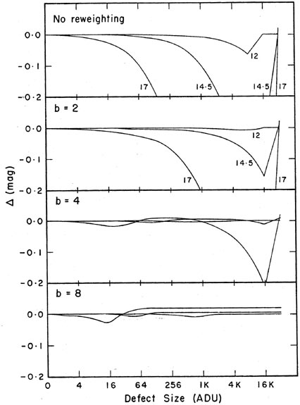
Finally, I would like to show the results of another quickie test I did to see whether the (a, b) weight-fudging scheme I talked about in my third lecture would help any. In one CCD frame, I chose three well-isolated stars of different apparent magnitudes, and performed profile fits on them. Then I simulated a cosmic-ray hit on the image by simply adding a certain brightness increment to that pixel which was closest to the center of the star. I repeated this for "defects" of increasing size, and watched how the derived magnitudes for the three stars changed with different amplitudes for the "cosmic-ray" event. This experiment is represented in the uppermost panel of Fig. 4-7. The brightest star, with an instrumental magnitude of ~ 12, is only about a factor of two fainter than a star which would have saturated the CCD; thus, it is among the brightest stars that one would want to measure. Then there is another star a factor of 10 fainter, with an instrumental magnitude of 14.5; and finally a third star ten times fainter again, with an instrumental magnitude of 17, which is maybe a factor of two brighter than the faintest star you could reliably detect in this image. As you can see, adding arbitrary amounts of flux to these stars makes them all brighter (surprise!), and the faintest star gets brighter faster than the brightest one (surprise, surprise!). As the "cosmic-ray event" get stronger, the magnitude errors grow until the point is reached where the defect crosses over the "maximum good data-value" threshold, and the answer switches abruptly to the best profile fit based on all the pixels within the fitting region except the corrupted one. The other three panels show how the magnitudes resulting from the best fit vary with defect size, for a = 2.5 and b = 2, 4, and 8. As you can see, increasing b reduces the size of the maximum error that a cosmic-ray hit can produce in the photometric result, and it also reduces the size of the discontinuous jump in the derived magnitude that will be produced by a tiny increase in the size of the cosmic ray event (viz., that increment which changes it from a "good" pixel to a "bad" one). For a = 2.5 and b = 8, the maximum error produced by a cosmic-ray hit on the faintest star is only 0.025 mag - and this in a star which is already uncertain by about 0.025 mag because of readout noise and Poisson statistics alone. In my opinion, since we know that the error sources in a CCD image are not strictly Gaussian (cosmic rays, hot pixels, electron traps, flat-field errors, undected stars can all be comparable to or larger than readout noise and photon statistics in individual pixels - especially when many consecutive frames are averaged into one) one should not stand upon arguments of mathematical purity and insist upon cookbook least squares. You'll probably get better answers if your program (gently) withdraws some of its confidence from funny-looking data.
|
| Figure 4-7. |
This assertion is patently not true when the data are undersampled. When
you are
trying to determine three or four fitting parameters for a star image
which may only occupy
four or five pixels, it's foolish to give the computer permission to
throw away any pixel it
doesn't like. You have to be more subtle here. One possibility is to
shade  toward a value
of 1.0, so large residuals don't get ignored, they get
medianed. Otherwise, it's probably
better to turn the clipping off altogether and accept the fact that
you'll get total garbage
(as distinguished from partial garbage) for some of your stars. I think
that someday there
will be a more sophisticated solution, which is this: when multiple
exposures of a given field
are available, all exposures will be reduced simultaneously. Let's say
you've got eight frames
of a field, with sampling such that each star occupies, on average, four
pixels. Now you've
got 32 data points to use in determining the star's 3 unknowns - its (x,
y) centroid and its
magnitude; 10 unknowns if you think the star may be a variable. Now it's
probably safe
to throw away cosmic-ray hits. In the best of all possible worlds, the
eight frames would
be subject to arbitrary translations and rotations with respect to one
another: that keeps
the star from always falling on the same detector flaws, and it gives
new information on
exactly what the star's position is by sampling the profile a little
differently each time. Now
you've got 35 new unknowns - the four transformation constants that
relate the coordinate
systems of each of frames 2, ... , 8 to that of frame 1 (see
Lectures 1
and 5), and the one
constant to relate the photometric zero point of each of the subsequent
frames to the system
of the first - but there are N stars in the field! You've got 4 x
N x 8 observations (four
pixels per star per frame to solve for 3N + 35 unknowns (plus an
additional 7 magnitudes
for each of the suspected variable stars) - you're gloriously overdetermined!
toward a value
of 1.0, so large residuals don't get ignored, they get
medianed. Otherwise, it's probably
better to turn the clipping off altogether and accept the fact that
you'll get total garbage
(as distinguished from partial garbage) for some of your stars. I think
that someday there
will be a more sophisticated solution, which is this: when multiple
exposures of a given field
are available, all exposures will be reduced simultaneously. Let's say
you've got eight frames
of a field, with sampling such that each star occupies, on average, four
pixels. Now you've
got 32 data points to use in determining the star's 3 unknowns - its (x,
y) centroid and its
magnitude; 10 unknowns if you think the star may be a variable. Now it's
probably safe
to throw away cosmic-ray hits. In the best of all possible worlds, the
eight frames would
be subject to arbitrary translations and rotations with respect to one
another: that keeps
the star from always falling on the same detector flaws, and it gives
new information on
exactly what the star's position is by sampling the profile a little
differently each time. Now
you've got 35 new unknowns - the four transformation constants that
relate the coordinate
systems of each of frames 2, ... , 8 to that of frame 1 (see
Lectures 1
and 5), and the one
constant to relate the photometric zero point of each of the subsequent
frames to the system
of the first - but there are N stars in the field! You've got 4 x
N x 8 observations (four
pixels per star per frame to solve for 3N + 35 unknowns (plus an
additional 7 magnitudes
for each of the suspected variable stars) - you're gloriously overdetermined!
6 Actually, you can fit the local sky
brightness with more than one parameter, and
some software packages routinely do. For instance, if your stars are in
a globular
cluster or superimposed on an elliptical galaxy or something, you can
replace B with
B0 + Bx(x -
x0) + By(y -
y0), and solve for the three parameters B0,
Bx, By, thereby
fitting a least-squares plane to the background. There's no theoretical
reason why you have
to stop here; if the data were good enough you could fit polynomial
surfaces of arbitrary
order, or segments of Hubble laws, or whatever you like.
Back.