Suppose we were to toss an unbiased coin 4 times in succession. What is the probability, P(k), of obtaining k heads? There are 16 different ways the coins might land; each is equally probable. Let's write down all 16 but group them according to how many heads appear, using the binary notation 1 = heads, 0 = tails:
| Sequence | No. heads | P(k) |
| 0000 | 0 | P(0) = 1/16 |
| 1000 | 1 | |
| 0100 | 1 | P(1) = 4/16 = 1/4 |
| 0010 | 1 | |
| 0001 | 1 | |
| 1100 | 2 | |
| 1010 | 2 | |
| 1001 | 2 | |
| 0110 | 2 | P(2) = 6/16 = 3/8 |
| 0101 | 2 | |
| 0011 | 2 | |
| 1110 | 3 | |
| 1101 | 3 | |
| 1011 | 3 | P(3) = 4/16 = 1/4 |
| 0111 | 3 | |
| 1111 | 4 | P(4) = 1/16 |
From Eq. A. 1, the probability of a given sequence is 1/16. From Eq. A.2, the probability of obtaining the sequence 1000, 0100, 0010, or 0001, i.e., a sequence in which 1 head appears, is 1/16 + 1/16 + 1/16 + 1/16 = 1/4. The third column lists these probabilities, P(k).
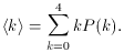
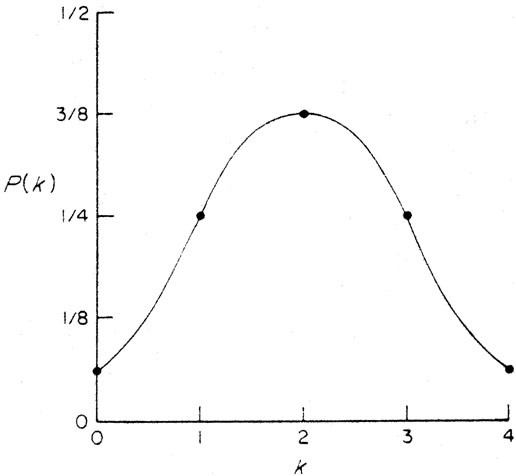
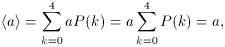
The results of these calculations can be summarized by plotting P(k) as a function of k, as shown in Fig. A.1. Such a plot is called a theoretical probability distribution. The peak value, k = 2, is the most probable value. Since the curve is symmetric about k = 2, this value also must be the mean value. One can compute the mean or expectation value of k by adding the number of heads obtained for each of the sequences shown in the table and dividing by 16, or - and this is the same thing - by weighting each possible value of k by the probability of obtaining that value, P(k), and computing the sum:
Figure A.1. The probability, P(k),
of obtaining k heads in 4 tosses of
an unbiased coin. This theoretical probability distribution is
discrete;
it is defined only for the integer values k = 0, 1, 2, 3, or
4. A smooth
line is drawn through the points only to make it easier to visualize the
trend. The distribution has a mean value 2 and a standard deviation 1.
The value of this sum is (0)(1/16) + (1)(1/4) + (2)(3/8) +
(3)(1/4) + (4)(1/16) = 0 + 1/4 + 3/4 + 3/4 + 1/4 = 2, as
expected. Note that
The probability of obtaining 0, 1, 2, 3, or 4 heads is 1. The
distribution is properly normalized.
Note also that if a is a constant (does not depend on the
variable k),
and
It is useful to have some measure of the width or spread
of a distribution about its mean. One might compute
<k - µ>, the expectation value of the deviation of k from
the mean µ = <k>, but the answer always comes out 0. It
makes more sense to compute the expectation value of the
square of the deviation, namely
This quantity is called the variance. Its square root,
where
For the distribution of Fig. A.1,
<k2> = (0)(1/16) + (1)
(1/4) + (4)(3/8) + (9)(1/4) + (16)(1/16) = 0 + 1/4 + 6/4
+ 9/4 + 1 = 5, <k>2 = 4, and
It is instructive to sit down and actually flip a coin 4
times in succession, count the number of heads, and then
repeat the experiment a large number of times. One can
then construct an experimental probability distribution,
with P(0) equal to the number of experiments that give 0
heads divided by the total number of experiments, P(1)
equal to the number of experiments that give 1 head
divided by the total number of experiments, etc. Two
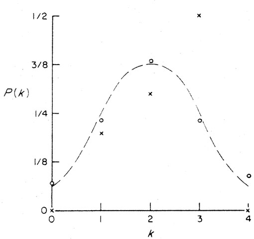
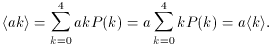
such distributions are shown in Fig. A.2. In the
first (x), the total number of experiments was 10. In the second (o),
the total number was 100.
Figure A.2. Two experimental probability
distributions. In one (x), a
coin was flipped 4 times in 10 successive experiments; the mean value
is 2.30, the standard deviation is 1.22. In the other (o), a coin was
flipped 4 times in 100 successive experiments; the mean value is 2.04,
the standard deviation 1.05. The dashed curve is the theoretical
probability distribution of Fig. A.1.
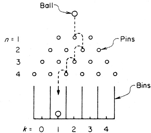
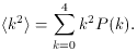
If you do not like flipping coins, you can build a
probability machine of the sort shown in
Fig. A.3. If the
machine is level and well made, the probability that a ball
bounces to the right or the left on striking the next pin is
1/2. The number of successive trials is equal to the
number of rows of pins. If you drop 100 balls through this
machine, they will pile up in the bins at the bottom, forming
a distribution like the one shown in
Fig. A.2. Or do the
experiments on a computer: ask for a random number
uniformly distributed between 0 and 1; if the number is
less than or equal to 1/2, call it a head; if it is greater than
1/2, call it a tail. The data shown in Fig. A.2 were
generated in this way.
The theoretical expectations are more closely met the
larger the number of samples. What is the likelihood that
the deviations between the experimental distributions and the
theoretical distribution, evident in Fig. A.2,
occur by chance? By how much are the mean values of the experimental
distributions likely to differ from the mean value
predicted by the theory? Questions of this kind often are
encountered in the laboratory. They are dealt with in
books on data reduction and error analysis and will not be
pursued here.
Figure A.3. A probability machine of 4
rows. A ball dropped on the
center pin of the top row bounces to the right or left and executes a
random walk as it moves from row to row, arriving finally at one of
the bins at the bottom. The rows and bins are numbered n = 1, 2, 3, 4
and k = 0, 1, 2, 3, 4, respectively; n is the bounce
number and k is the
number of bounces made to the right.


 ,
is called the standard deviation. Since µ = <k> and
µ2 = <k>2 are constants,
Eq. A.13 can be simplified. It follows from Eqs. A.11 and A.12 that
,
is called the standard deviation. Since µ = <k> and
µ2 = <k>2 are constants,
Eq. A.13 can be simplified. It follows from Eqs. A.11 and A.12 that

 2 = 5 - 4 = 1.