


Three distinct techniques for the measurement of the Sunyaev-Zel'dovich
intensity effects in clusters of galaxies are now yielding reliable
results. This section reviews single-dish radiometric
observations, bolometric observations, and interferometric
observations of the effects,
emphasizing the weaknesses and strengths of each technique and the types of
systematic error from which they suffer. A discussion of the
constraints on observation of the non-thermal effect is contained in
the discussion of bolometric techniques. No concerted efforts at
measuring the polarization Sunyaev-Zel'dovich effects have yet been
made, and so only
intensity-measuring techniques will be addressed here.
8.1.
Single-dish radiometer measurements
The original technique used to detect the Sunyaev-Zel'dovich effects made use of existing radio telescopes on which large tranches of observing time could be obtained. This always meant the older single-dish telescopes, so that the measurements were made using traditional radiometric methods. This is exemplified by the early work of Gull & Northover (1976) using the Chilbolton 25-m telescope, or the more recent work of Uson (1986) on the NRAO 140-foot telescope. These telescopes tend to have beam-sizes of a few arcminutes at microwave frequencies, which is a fairly good match to the angular sizes of the moderately distant clusters of galaxies which X-ray astronomy was then beginning to study. With such large and general-purpose telescopes, it was impossible to make major modifications that would optimize them for observations of the microwave background radiation, and much early work had to cope with difficulties caused by the characteristics of the telescopes through minor changes to the receiver package or careful design of the observing strategy.
The closest clusters of galaxies (at redshifts less than about 0.05) have larger angular sizes, and it is possible to observe the Sunyaev-Zel'dovich effects using smaller telescopes. In such cases is has been possible to rework existing antennas to optimize them for microwave background observations - both of the Sunyaev-Zel'dovich effects and primordial structures (for example, using the OVRO 5.5-m telescope; Myers et al. 1997). This is now leading to a generation of custom-designed telescopes for sensitive measurements of the CMBR: some ground-based and some balloon-based systems should be in use in the near future.
A simple estimate of the sensitivity of a single-dish observation is of interest. A good system might have a noise temperature of about 40 K (including noise from the atmosphere) and a bandwidth of 1 GHz. Then in 1 second, the radiometric accuracy of a simple measurement will be 0.9 mK, and a differenced measurement, between the center of a cluster of galaxies and some reference region of blank sky, would have an error of 1.3 mK. Thus if problems with variations in the atmosphere are ignored, it would appear that a measurement with an accuracy of 10 µK could be made in 4.4 hours.
This observing time estimate is highly optimistic, principally because of emission from the Earth's atmosphere. Sensitive observations with large or small single dishes always use some differencing scheme in order to reduce unwanted signals from the atmosphere (or from the ground, appearing in the sidelobes of the telescope) to below the level of the astronomical signal that is being searched for. Consider, for example, observations at 20 GHz, for which the atmospheric optical depth may be ~ 0.01 in good conditions at a good site. The atmospheric signal will then be of order 3 K, several thousand times larger than the Sunyaev-Zel'dovich effects, and atmospheric signals must be removed to a part in 105 if precise measurements of the Sunyaev-Zel'dovich effects are to be made.
The simplest scheme for removing the atmospheric signal is simply to position-switch the beam of an antenna between the direction of interest (for example the center of some cluster) and a reference direction well away from the cluster. The radiometric signals measured in these two directions are then subtracted. If the atmospheric signal has the same brightness at the cluster center as at the reference position, then it is removed, and the difference signal contains only the astronomical brightness difference between the two positions. Thus the reference position is usually chosen to be offset in azimuth, so that the elevations and atmospheric path lengths of the two beams are as similar as possible.
Of course, the sky in the target and reference directions will be different because of variations in the properties of the atmosphere with position and time, and because of the varying elevation of the target as it is tracked across the sky. Nevertheless, if the target and reference positions are relatively close together, the switching is relatively fast, and many observations are made, it might be expected that sky brightness differences between the target and reference positions would average out with time. The choice of switching angle and speed is made to try to optimize this process, while not spending so much time moving the beams that the efficiency of observation is compromised.
An alternative strategy is to allow the sky to drift through the beam of the telescope or to drive the telescope so that the beam is moved across the position of the target. The time sequence of sky brightnesses produced by such a drift or driven scan is then converted to a scan in position, and fitted as the sum of of a baseline signal (usually taken to be a low-order polynomial function of position) and the Sunyaev-Zel'dovich effect signal associated with the target. Clearly, structures in the atmosphere will cause the baseline shape to vary, but provided that these structures lie on scales larger than the angular scale of the cluster, they can be removed well by this technique. Many scans are needed to average out the atmospheric noise, and this technique is often fairly inefficient, because the telescope observes baseline regions far from the cluster for much of the time.
In practice these techniques are unlikely to be adequate, because of the amplitude of the variations in brightness of the atmosphere with position and time: at most sites the sky noise is a large contribution to the overall effective noise of the observation. Nevertheless, the first reported detection of a Sunyaev-Zel'dovich effect (towards the Coma cluster, by Parijskij 1972) used a simple drift-scanning technique, with a scan length of about 290 arcmin and claimed to have measured an effect of -1.0 ± 0.5 mK.
More usually a higher-order scheme has been employed. At cm wavelengths, it is common for the telescope to be equipped with multiple feeds so that two or more directions on the sky can be observed without moving the telescope. The difference between the signals entering through these two feeds is measured many times per second, to yield an ``instantaneous'' beam-switched sky signal. On a slower timescale the telescope is position-switched, so that the sky patch being observed is moved between one beam and the other. At mm wavelengths it is common for the beam switching to be provided not by two feeds, but by moving the secondary reflector, so that a single beam is moved rapidly between two positions on the sky. This technique would allow complicated differencing strategies, if the position of the secondary could be controlled precisely, but at present only simple schemes are being used. Arrays of feeds and detectors are now in use on some telescopes, and differencing between signals from different elements of these feed arrays also provide the opportunity for new switching strategies (some of which are already being used in bolometer work, see Sec. 8.2).
| Paper | Technique | 
|  h
h
| b
| s
| |
| (GHz) | (arcmin) | (arcmin) | (arcmin) | |||
| Parijskij 1972 | DS | 7.5 | 1.3 x 40 | . . . | 290 | |
| Gull & Northover 1976 | BS+PS | 10.6 | 4.5 | 15.0 | . . . | * |
| Lake & Partridge 1977 | BS+PS | 31.4 | 3.6 | 9.0 | . . . | * |
| Rudnick 1978 | BS+DS | 15.0 | 2.2 | 17.4 | 60-120 | |
| Birkinshaw et al. 1978a | BS+PS | 10.6 | 4.5 | 15.0 | . . . | * |
| Birkinshaw et al. 1978b | BS+PS | 10.6 | 4.5 | 15.0 | . . . | * |
| Perrenod & Lada 1979 | BS+PS | 31.4 | 3.5 | 8.0 | . . . | |
| Schallwich 1979 | BS+DS | 10.7 | 1.2 | 8.2 | 15 | * |
| Lake & Partridge 1980 | BS+PS | 31.4 | 3.6 | 9.0 | . . . | |
| Birkinshaw et al. 1981a | BS+PS | 10.7 | 3.3 | 14.4 | . . . | * |
| Birkinshaw et al. 1981b | BS+PS | 10.6 | 4.5 | 15.0 | . . . | |
| Schallwich 1982 | BS+DS | 10.7 | 1.2 | 8.2 | 15 | |
| Andernach et al. 1983 | BS+DS | 10.7 | 1.2 | 3.2, 8.2 | 15 | |
| Lasenby & Davies 1983 | BS+PS | 5.0 | 8 x 10 | 30 | . . . | |
| Birkinshaw & Gull 1984 | BS+PS | 10.7 | 3.3 | 20.0 | . . . | |
| BS+PS | 10.7 | 3.3 | 14.4 | . . . | ||
| BS+PS | 20.3 | 1.8 | 7.2 | . . . | ||
| Birkinshaw et al. 1984 | BS+PS | 20.3 | 1.8 | 7.2 | . . . | |
| Uson & Wilkinson 1984 | BS+PS | 19.5 | 1.8 | 8.0 | . . . | * |
| Uson 1985 | BS+PS | 19.5 | 1.8 | 8.0 | . . | * |
| Andernach et al. 1986 | BS+DS | 10.7 | 1.18 | 3.2, 8.2 | 15 | |
| Birkinshaw 1986 | BS+PS | 10.7 | 1.78 | 7.15 | . . | * |
| Birkinshaw & Moffet 1986 | BS+PS | 10.7 | 1.78 | 7.15 | . . . | * |
| Radford et al. 1986 | BS+DS | 90 | 1.3 | 4.0 | 10 | |
| BS+PS | 90 | 1.2 | 4.3 | . . . | ||
| BS+PS | 105 | 1.7 | 19 | . . . | ||
| Uson 1986 | BS+PS | 19.5 | 1.8 | 8.0 | . . . | * |
| Uson & Wilkinson 1988 | BS+PS | 19.5 | 1.8 | 8.0 | . . . | |
| Birkinshaw 1990 | BS+PS | 20.3 | 1.78 | 7.15 | . . . | * |
| Klein et al. 1991 | BS+DS | 24.5 | 0.65 | 1.90 | 6.0 | |
| Herbig et al. 1995 | BS+PS | 32.0 | 7.35 | 22.16 | . . . | |
| Myers et al. 1997 | BS+PS | 32.0 | 7.35 | 22.16 | . . . | |
| Uyaniker et al. 1997 | DS | 10.6 | 1.15 | . . . | 10 | |
| Birkinshaw et al. 1998 | BS+PS | 20.3 | 1.78 | 7.15 | . . . | |
| Tsuboi et al. 1998 | BS+PS | 36.0 | 0.82 | 6.0 | . . . | |
| Note. - The technique codes are BS for beam-switching, PS for
position-switching, DS for drift- or driven-scanning. is the
central frequency of observation. h is the FWHM of the
telescope. b is the beam-switching angle (if
beam-switching was used), and s is the scan length (for
drift or driven scans). * in the final column indicates that the
paper contains data that are also included in a later paper in the
Table.
| ||||||
Table 1, which reports the critical observing
parameters used in all
published radiometric observations of the Sunyaev-Zel'dovich effects,
indicates the switching scheme that was used. Most measurements have been made
using a combination of beam-switching (BS) and position-switching
(PS), because this is relatively efficient, with about half the
observing time being spent on target. Some observations, including all
observations by the
Effelsberg group, have used a combination of beam-switching and drift
or driven scanning (DS). The critical parameters of these techniques
are the telescope beamwidth (the full width to half maximum, FWHM),
h, the beam-switching
angle, b, and the
angular length of the drift or driven scan, s. Some of
the papers in Table 1 have been partially or fully
superseded by later papers, and are marked *.

Figure 13. A representative beam and position-switching scheme, and background source field: for observations of a point near the center of Abell 665 by the Owens Valley Radio Observatory 40-m telescope. The locations of the on-source beam and reference beams in this symmetrical switching experiment are shown as solid circles. The main beam is first pointed at the center of the cluster with the reference beam to the NW while beam-switched data are accumulated. The position of the main beam is then switched to the SE offset position, with the reference beam pointed at the center of the cluster, and more beam-switched data are accumulated. Finally, the main beam is again pointed at the cluster center. As the observation extends in time, the offset beam locations sweep out arcs about the point being observed, with the location at any one time conveniently described by the parallactic angle, p. Since Abell 665 is circumpolar from the Owens Valley, the reference arcs close about the on-source position: however, the density of observations is higher at some parallactic angles because p is not a linear function of time (see equation 91). |
In techniques that use a combination of beam-switching and position
switching, the beam and position
switching directions need not be the same, and need
bear no fixed relationship to any astronomical axes. However, the
commonest form of this technique (illustrated in
Fig. 13) has the telescope equipped with a twin-beam
receiver with the two beams offset in azimuth. Since large
antennas are usually altazimuth mounted, it is convenient also to
switch in azimuth (and so keep the columns of atmosphere roughly
matched between the beams). In any one
integration interval (typically some fraction of a second) the output
of the differential radiometer is proportional to the brightness
differences seen by the two beams (possibly with some offset because
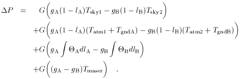
of differences in the beam gains, losses, etc.). The configuration used by
Readhead et al.
(1989)
in their observations of primordial
anisotropies in the microwave background radiation is typical. In the
simplest arrangement, where the two beams (A and B) are pointed towards
sky positions 1 and 2, and the signals from the feeds enter
a Dicke switch, followed by a
low-noise front-end receiver, and then are synchronously detected by a
differencing backend, the instantaneous output of the radiometer,
 P, was written by
Readhead et al. as
P, was written by
Readhead et al. as
Here G is the gain of the front-end system (a maser in the OVRO
40-m telescope configuration used by Readhead et al.), with an
equivalent noise temperature of
Tmaser. gA and
gb are the back-end gains corresponding to the A and B (main
and reference) feeds, and lA and
lb are the losses
in the feeds, waveguides, and Dicke switch associated with the two
channels. These losses are distributed over a number of components,
with temperatures
It is clear that the instantaneous difference power between channels A
and B may arise from a number of causes other than the sky temperature
difference (Tsky1 - Tsky2) which it
is desired to
measure. In general, the atmospheric signal greatly exceeds the
astronomical signal towards any one position on
the sky (Tatm1 >> Tsky1) so that small
imbalances in the atmospheric signal between the two beams dominate
over the astronomical signals that are to be measured. Over
long averaging times, and with the same zenith angle coverage in the
two beams, it is expected that < Tatm1 -
Tatm2 >
The ground pickup signals through the two beams are likely to be
different, since the detailed shapes of the telescope beams are also
different. This leads to an imbalance TgndA -
TgndB, and
an offset signal in the radiometer. The amplitude of this signal is
reduced to a minimum by tapering the illumination of the primary
antenna, so that as little power as possible arrives at the feed from
the ground. Some protection against ground signals is also achieved by
operating at elevations for which the expected spillover signal is
smallest. However, since the ground covers a large solid angle
there are inevitably reflection and diffraction effects that cause
offsets from differential ground spillover.
The losses lA and lb in the two
channels of the
radiometer are reduced to a minimum by keeping the waveguide lengths
to a minimum and using the best possible microwave components,
but it is impossible to ensure that the losses are equal. Furthermore, the
temperatures of the components in which these losses occur depend
critically on where they are in the radiometer housing, so that the
radiated signals from the components,
These problems are exacerbated by their time variations. It is likely
that the gains and temperatures will drift with time. The receiver
parameters are stabilized as well as possible, but are still
seen to change slowly. The atmosphere and ground pickup temperatures
change more significantly, with varying weather conditions and
varying elevations of the observation. Thus simple beam-switched
measurements of the Sunyaev-Zel'dovich effect are unlikely to be
successful, even after filtering out periods of bad weather and rapid
temperature change when the atmospheric signal is unstable.
The level of differencing introduced by position-switching removes many
of these effects to first order in time and position on the sky. The
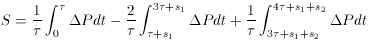
standard position-switching technique points one beam (A, the ``main
beam'') at the target position for time
is a much better measurement of the sky temperature difference
between the target and the average of two points to either side of it
(offset in azimuth by the beam-switching angle,
Even at this degree of differencing, it is important to check that the
scheme is functioning properly. For this reason, the best work has
included either a check of regions of nominally blank sky near the
target point, or a further level of differencing involving the
subtraction of data from fields leading and following the target field
by some interval. A representative method
(Herbig et al.
1995)
consists of
making a few (~ 10) observations using the beam-switching plus
position switching technique described above at the target field,
referenced to the same number of observations on offset regions
before and after the target field, with the time interval arranged so
that the telescope
moves over the same azimuth and elevation track as the target
source. The off-target data may be treated as controls, or may be
directly subtracted from the on-target data to provide another level
of switching which is likely to reduce the level of differential
ground spillover. In either case, rigorous controls of this type
necessarily reduce the efficiency of the observations by a factor 2
or 3. Alternatively, observations can be made of closer positions
(perhaps even overlapping with the reference fields of the target
point), without attempting an exact reproduction of the azimuth and
elevation track on any one day, but allowing an equal coverage to
build up over a number of days. This was the approach used by
Birkinshaw et
al. (1998).
The various beam switching schemes that have been used are described
in detail in the papers in Table 1 that discuss
substantial blocks of measurements. Quantitative estimates of their
systematic errors from differential ground spillover, residual
atmospheric effects, or receiver drifts, are also usually given.
Whichever beam-switching technique is used, it is advisable to use the
same technique to
observe control fields, far from known X-ray clusters, where the
expected measurement is zero. Systematic errors in the technique are
then apparent, as is the extra noise in the data caused by primordial
structures in the CMBR. It is important to realize
that the Sunyaev-Zel'dovich effect plus primordial signal at some point can
be measured to more precision than the systematic error on the
Sunyaev-Zel'dovich
effect that is set by the underlying spectrum of primordial
fluctuations. That is, the measurement error is a
representation of the reproducibility of the measurement, which is the
difference between the brightness of some point relative to a weighted
average of adjacent points. Noise from the spectrum of primordial
fluctuations must be taken into account if realistic
errors on physical parameters of a cluster are to be deduced from
measured Sunyaev-Zel'dovich effect data.
A further difficulty encountered with single-dish observations is that
of relating the measured signal from the radiometer (in volts, or
some equivalent unit) to the brightness temperature of a
Sunyaev-Zel'dovich effect on the sky. The opacity of the atmosphere can be
corrected using tip measurements, and generally varies little during
periods of good weather, so that the principal problem is not one of
unknown propagation loss but rather one of calibration. Generally the absolute
calibration of a single-dish system is tied to observations of
planets, with an internal reference load in the radiometer being
related to the signal obtained from a planet. If that planet has solid
brightness temperature Tp, then the output signal is
proportional to Tp, with a constant of proportionality which
depends on the solid angle of the planet, the telescope beam pattern,
etc. Thus by measuring the telescope beam pattern and the signal from
planets, it is possible to calibrate the internal load. The accuracy
of this calibration is only modest because of
Thus, for example, the recent measurements of Myers
et al. (1997) are
tied to a brightness temperature scale using the measurement of the
brightness temperature of Jupiter at 18.5 GHz
(Wrixson et al. 1971).
This measurement may itself be in
error by up to 6 per cent. Difficulties may also arise from changes in
the internal reference load, which will cause the
calibration to drift with time. Relating this load back to sky
temperatures at a later date will introduce another set of ``transfer
errors''. Even if these are well controlled, it is clear that
radiometric Sunyaev-Zel'dovich effect data contain systematic
uncertainties in the
brightness scale at the 8 per cent level or worse. This calibration
error has a significant effect on the interpretation of the results.
It is important to mention, at this stage, that the differencing
schemes described here have the effect of restricting the range of
redshifts for which the telescope is useful. If observations are to be
made of a cluster of galaxies at low redshift, then the angular size
of the cluster's Sunyaev-Zel'dovich effects (which are several times
larger than of
the cluster's X-ray surface brightness) may be comparable to the
beam-switching angle,
In dealing with the variations of signal during a tracked observation
of a cluster, it is convenient to introduce the concept of parallactic
angle, the angle between the vertical circle and the declination
axis. An observation at hour angle H of a source at declination
where the parallactic angle increases from negative values to positive
values as time increases (with the parallactic angle being zero at
transit; Fig. 13) for sources south of the telescope,
and decreases from positive values to negative values for sources
north of the
telescope. For a symmetrical beam-switching experiment, like that
depicted in Fig. 13, the parallactic angle may be
taken to lie in
-90° to +90°. With more complicated beam-switching
schemes, which may be asymmetrical to eliminate higher-order terms
in the time or position dependence (e.g.,
Birkinshaw & Gull 1984),
the full range of p may be needed.
The conversion between time and parallactic
angle is particularly convenient when it is necessary to
keep track of the radio source contamination. Many of the observations
listed in Table 1 were made at cm wavelengths,
where the atmosphere is relatively benign and large antennas are
available for long periods. However, the radio sky is then
contaminated by non-thermal sources associated with galaxies (in the
target cluster, the foreground, or the background) and quasars, and
the effects of these radio sources must be subtracted if the
Sunyaev-Zel'dovich effects are to be seen cleanly.
Figure 15 shows a map of the radio sky near
Abell 665. Significant radio source emission can be
found in the reference arcs of the observations at
many parallactic angles. Such emission causes
the measured brightness temperature difference between the center and
edge of the cluster to be negative: a fake Sunyaev-Zel'dovich effect is
generated. Protection against such fake effects is implicit in the
differencing scheme. Sources in the reference arcs affect
the Sunyaev-Zel'dovich effect measurements only for the range of
parallactic angles that
the switching scheme places them in the reference beam. A plot of
observational data arranged by parallactic angle therefore shows
negative features at parallactic angles corresponding to radio source
contamination (e.g., Fig. 16), and data near these
parallactic angles can be corrected for the contamination using radio
flux density measurements from the
VLA, for example.
This procedure is further complicated by issues of source
variability. At frequencies above 10 GHz where most radiometric
observations are made (Table 1), many of the brightest
radio sources are variable with timescales of months being
typical. Source subtraction based on archival data is therefore
unlikely to be good enough for full radiometric accuracy to be
recovered. Simultaneous, or near-simultaneous, monitoring of variable
sources may then be necessary if accurate source subtraction is to be
attempted, and this will always be necessary for variable sources
lying in the target locations. Variable sources lying in the
reference arcs may also be simply eliminated from consideration by
removing data taken at the appropriate parallactic angles: thus in
Fig. 16, parallactic angle ranges near -50°
and +40° might be eliminated on the basis of variability or of
an imprecise knowledge of the contaminating sources. However, sources
which are so strongly variable that they appear from below the flux
density limit of a radio survey will remain a problem without adequate
monitoring of the field.
Despite difficulties with radio source contamination, calibration, and
systematic errors introduced by the radiometer or spillover,
recent observations of the Sunyaev-Zel'dovich effects using radiometric
techniques
are yielding significant and
highly reliable measurements. The detailed results and critical
discussion appear in Sec. 9, but a good
example is the
measurement of the Sunyaev-Zel'dovich effect of the Coma cluster by
Herbig et al.
(1995),
using
the OVRO 5.5-m
telescope at 32 GHz. Their result, an antenna
temperature effect of -175 ± 21 µK, corresponds to a
central Sunyaev-Zel'dovich effect
For a few clusters, single-dish measurements have been used not only
to detect the central decrements, but also to measure the angular
sizes of the effects. This is illustrated in Fig. 17
which, for the
three clusters CL 0016+16, Abell 665, and Abell 2218 shows the
Sunyaev-Zel'dovich effect
results of
Birkinshaw et
al. (1998).
The close agreement
between the centers of the Sunyaev-Zel'dovich effects and the X-ray
images of the
clusters is a good indication that the systematic problems of
single-dish measurements have been solved, although
observing time limitations and the need to check for systematic
errors restricts this work to a relatively coarse measurement
of the cluster angular structure. Much better results should be
obtained using two-dimensional arrays of detectors, as should be
available on the Green Bank Telescope when it is completed.
 (89)
(89)
 A
and B which range
from the cryogenic temperatures of the front-end system to the ambient
temperatures of the front of the feeds.
A
and B which range
from the cryogenic temperatures of the front-end system to the ambient
temperatures of the front of the feeds.
 0. The accuracy with which this is true will depend
on the weather patterns at the telescope, the orientation of the beams
relative to one another, and so on.
0. The accuracy with which this is true will depend
on the weather patterns at the telescope, the orientation of the beams
relative to one another, and so on.
 A dlA
and B dlB
are likely to be significantly different. Once again, this produces an
offset signal between the two sides of the radiometer.
A dlA
and B dlB
are likely to be significantly different. Once again, this produces an
offset signal between the two sides of the radiometer.
 , with the second beam
(B, the ``reference beam'') offset in azimuth to some reference
position, then switches the reference beam onto the target for time 2
, with the main beam offset to a
reference position on the
opposite side of the target, then switches back for a final time
with the original beam on the
target. If the total cycle time
(4 + s1 +
s2, where s1 and
s2 are the times spent
moving) is small, then the reference positions observed by beams A and
B do not change appreciably during a cycle, and the combination
, with the second beam
(B, the ``reference beam'') offset in azimuth to some reference
position, then switches the reference beam onto the target for time 2
, with the main beam offset to a
reference position on the
opposite side of the target, then switches back for a final time
with the original beam on the
target. If the total cycle time
(4 + s1 +
s2, where s1 and
s2 are the times spent
moving) is small, then the reference positions observed by beams A and
B do not change appreciably during a cycle, and the combination
 b) than
the estimate in (89). This is so even when
the move and dwell times in the different
pointing directions change slightly, for example because of variations
in windage on the telescope. If is
chosen to be small,
then quadratic terms in the time and position variations of
contaminating effects in (89) can be made very
small, but at the cost of much reduced efficiency
4 + s1 + s2) in the
switching cycle. For observations with
the OVRO 40-m
telescope made by
Readhead et al.
(1989)
and
Birkinshaw et
al. (1998),
was chosen to be
about 20 sec, and even large non-linear terms in the telescope
properties are expected to be subtracted to an accuracy of a few µ
K.
b) than
the estimate in (89). This is so even when
the move and dwell times in the different
pointing directions change slightly, for example because of variations
in windage on the telescope. If is
chosen to be small,
then quadratic terms in the time and position variations of
contaminating effects in (89) can be made very
small, but at the cost of much reduced efficiency
4 + s1 + s2) in the
switching cycle. For observations with
the OVRO 40-m
telescope made by
Readhead et al.
(1989)
and
Birkinshaw et
al. (1998),
was chosen to be
about 20 sec, and even large non-linear terms in the telescope
properties are expected to be subtracted to an accuracy of a few µ
K.
1.
measurement errors in the planetary signal, from opacity
errors in the measurement of the transparency of the atmosphere,
pointing errors in the telescope, etc.,
2.
uncertainties in the brightness temperature scale of the
planets, and in the pattern of brightness across their disks, and
3.
variations in the shape of the telescope beam (and hence
the gain) over the sky.
b, and beam-switching reduces the
observable signal. Alternatively, if the cluster is at high redshift,
then its angular size in the Sunyaev-Zel'dovich effects may be smaller
than the telescope FWHM,
h, and beam dilution will reduce the
observable signal. The two effects compete, so that for any telescope
and switching scheme, there is some optimum redshift band for
observation, and this band depends on the structures of cluster
atmospheres and the cosmological model. An example of a
calculation of this
efficiency factor, defined as the fraction of the central
Sunyaev-Zel'dovich effect from a cluster that can be observed with the
telescope,
is shown in Fig. 14 for the OVRO 40-m
telescope. The steep cutoff at small redshift represents
the effect of the differencing scheme, while the decrease of the
efficiency factor at large z arises from the slow variation of
angular size with redshift at z  0.5.
0.5.

Figure 14. The observing efficiency factor,  ,
as a function of redshift, for observations of clusters with core
radius 300 kpc and
,
as a function of redshift, for observations of clusters with core
radius 300 kpc and  = 0.67, using the
OVRO 40-m
telescope at 20 GHz and assuming h100 = 0.5
and q0 =
1/2. is defined to be the
central effect seen by the telescope divided by the true
amplitude of the Sunyaev-Zel'dovich effect, and measures the
beam-dilution and beam-switching reductions of the cluster signal.
The decrease in at
z > 0.15 is slow, so that these
observations would be sensitive to the Sunyaev-Zel'dovich effects
over a wide redshift range.
= 0.67, using the
OVRO 40-m
telescope at 20 GHz and assuming h100 = 0.5
and q0 =
1/2. is defined to be the
central effect seen by the telescope divided by the true
amplitude of the Sunyaev-Zel'dovich effect, and measures the
beam-dilution and beam-switching reductions of the cluster signal.
The decrease in at
z > 0.15 is slow, so that these
observations would be sensitive to the Sunyaev-Zel'dovich effects
over a wide redshift range.
 from a telescope at latitude
 will occur at
parallactic angle
will occur at
parallactic angle

Figure 15. Observing positions and radio sources in
the cluster Abell 665. The dark-grey circles represent the FWHMs
of
the primary pointing positions of the
Birkinshaw et
al. (1998)
Sunyaev-Zel'dovich effect
observations in the cluster, while the light-grey areas are the
reference arcs traced out by the off-position beams. A VLA 6-cm radio
mosaic of the cluster field is shown by contours. Note the appearance
of a significant radio source under the pointing position 4 arcmin
north of the cluster center. This source appears to be variable,
causing significant problems in correcting the data at that
location. Other radio sources appear near or within the reference
arcs, and cause contamination of some parts of the data.


Figure 16. A comparison of the observed and
modeled parallactic angle scans for OVRO 40-m data at a point
7 arcmin south of the nominal center of Abell 665. Two features are
seen in the observed data (left). These correspond to bright radio
sources which are seen in the reference arcs at parallactic angles
near -50° and 40° (position angles
+40° and -50° on Figs. 13
and 15). The model of the
expected signal based on VLA
surveys of the cluster
(Moffet & Birkinshaw
1989)
shows features of
similar amplitude at these parallactic angles, so that moderately good
corrections can be made for the sources. The accuracy of these
source corrections is questionable because of the
extrapolation of the source flux densities to the higher frequency of
the Sunyaev-Zel'dovich effect data and the possibility that the sources are
variable.
TT0 + TK0 = -510 °
110 µK,
and is a convincing measurement of the Sunyaev-Zel'dovich effect from
a nearby cluster of galaxies for which particularly good X-ray and
optical data exist (e.g.,
White et al. 1993).

Figure 17. Measurements of changes in the apparent brightness
temperature of the microwave background radiation as a
function of declination near the clusters CL 0016+16, Abell 665
and Abell 2218
(Birkinshaw et
al. 1998).
The largest
Sunyaev-Zel'dovich effect is seen at the point closest to
the X-ray center for each cluster (offset from the scan
center in the case of Abell 665), and the apparent angular
sizes of the effects are consistent with the predictions of
simple models based on the X-ray data. The horizontal lines delimit
the range of possible zero levels, and the error bars
include both random and systematic components.