2. THE METHOD

Gravitational lensing relies upon the propensity of light to follow null geodesics in curved spacetime. This means that if we try to fit the round peg that is the curved space around a mass M into the square hole that is the pre-relativity framework of Euclid, Newton, and Kant, then light rays will appear to be deflected through an angle

(2.1)

where b is the impact parameter. Now, an elementary calculation of this deflection angle, analogous to the calculation of the deflection of an ultrarelativistic electron passing by an atomic nucleus, gives precisely half this deflection. When one analyzes the general relativistic calculation, one finds that the other half of the deflection is directly attributable to the space curvature and that this is a peculiar prediction of general relativity. This prediction has been verified with a relative accuracy of ~ 0.001 in a measurement of the solar deflection (Lebach et al. 1995) and we can take this part of the theory for granted.

It turns out to be quite useful (and rigorously defensible), to use the Newtonian framework to think in terms of this "deflection" and to treat space as flat but endowed with an artificial refractive index

(2.2)

where () is the conventional Newtonian gravitational potential which -> 0 as r -> (Eddington 1919). (As < 0, the refractive index exceeds unity and rays are deflected toward potential wells.) This also implies that when photons travel along a ray, they will appear to travel slower than in vacuo and will take an extra time t_grav to pass by a massive object, where

(2.3)

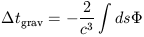
and where the integral is performed along the ray. (This effect is also known as the "Shapiro delay" and it has been measured with a fractional accuracy ~ 0.002 in the solar system by Reasenberg et al. 1979). If the deflector is at a cosmological distance (at a redshift z_d), the gravitational delay measured by the observer will be (1 + z_d) times longer, where the expansion factor takes into account the lengthening of time interval proportional to the lengthening of wave periods.

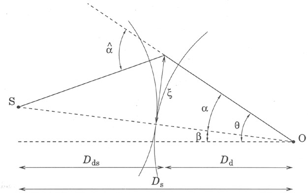
There is a second, geometrical contribution to the total time delay. In order to compute this contribution, it is necessary to take account of the fact that the global geometry of the universe is not necessarily flat. Fortunately, this can be done by defining an angular diameter distance (e.g. Weinberg 1972), which is the ratio of the proper size of a small source at the time of emission to the angle that it subtends at a distant observer. (In computing the angular diameter distance, it is necessary to allow for the fact that the universe expands as the light propagates from the source to the observer.) Now define angular diameter distances from the observer to the deflector and the source by D_d, D_s respectively and from the deflector to the source by D_ds. If we compare the true deflected ray with the unperturbed ray in the absence of the deflector, then elementary geometry tells us that the separation of the two rays at the deflector is given by = D_dD_ds / D_s (Fig. 1). Now imagine two waves, one emanating from the source at the time of emission, the other emanating from the observer backward in time leaving now and let these two waves meet tangentially at the deflector along the undeflected ray. The extra geometrical path is simply the separation of these wavefronts at the deflector along the deflected ray, a distance from the undeflected ray. As the rays are normal to the wavefronts at the deflector, we see that the geometrical path difference at the deflector is just . / 2. Again, we must multiply by (1 + z_d). The net result is an expression for the geometrical time delay

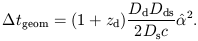
(2.4)

The total time delay is the sum of the gravitational and the geometrical contributions.

Both the gravitational and the geometrical time delays are of comparable magnitude ~ ² / H₀ for cosmologically distant sources. For typical deflections ~ 1", this would lead to an estimate t ~ 1 yr. Curiously, for many of the sources in which we are most interested, it turns out that the actual delays are much smaller than this estimate (by up to three orders of magnitude). This is because the gravitational and geometrical time delays tend to cancel each other out and because we tend to select observationally highly magnified examples of gravitational lensing in which the image arrangement is quite symmetrical.

Figure 1. Illustration of the geometrical time delay in a simplified lensing geometry. The two wavefronts shown in the figure represent one wave emanating from the source and the other wave emanating from the observer backward in time. They meet tangentially at the deflector along the undeflected ray. The separation between these two wavefronts along the deflected ray is given by the expression . / 2, regardless of the space curvature.

In order to evaluate Eqs. 2.3 and 2.4 in a given system, we must construct a model of the deflector. For a general mass distribution, the deflection angle, (which can be regarded as a two dimensional vector as long as it is small), is given by

(2.5)

where is a unit vector along the ray. We can now use this deflection to solve for the rays. Let us measure the angular position of the undeflected ray as seen by the observer relative to an arbitrary origin on the sky, by and the position of the deflected ray by (Fig. 1). These angles must satisfy the general lens equation

(2.6)

where

(2.7)

is the reduced deflection angle. When Eq. 2.6 has more than one solution, we have a strong gravitational lens producing multiple images. Common strong lenses form two or four images. We can use Eq. 2.6 to write the total time delay in the form

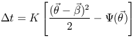
(2.8)

where

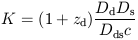
(2.9)

and

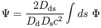
(2.10)

is the scaled surface potential which satisfies the two-dimensional Poisson equation

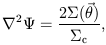
(2.11)

and where

(2.12)

is the reduced deflection angle. is the surface density in the lens plane and _c = c²D_s / 4 G D_ds D_d is the so-called critical density. The derivatives are performed with respect to .

Next, we must calculate the observed magnification. Suppose that we have a small but finite source that is resolved by the observer. In the absence of the deflector, the source will appear at position on the sky. After deflection, the plane will be mapped onto the plane. The Hessian tensor

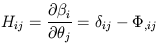
(2.13)

relates the source to the image. (Note that, as the deflection is itself the gradient of a potential, this tensor is symmetric and only has three independent components.) It is usual to relate the image to the source and this requires the magnification tensor which is the inverse of Eq. 2.13:

(2.14)

This magnification tensor can be decomposed into an isotropic expansion and a trace-free pure shear. As it is symmetric, there is no rotation.

Now the usual scalar magnification, denoted by µ, is the ratio of the flux observed from an unresolved source seen through the deflector to the flux that would have been measured in the absence of the deflector. As the intensity is unchanged by the deflector, this ratio is simply the ratio of the solid angles subtended by the ratio of the flux with and without lensing, given by the Jacobian

(2.15)

These magnifications are not directly observable. Rather, it is the ratio of the magnifications of separate images of the same source that one measures. (Of course this may have to be done at different times of observation if the source varies so as to make the comparison at the same time of emission.) Similarly, if we are able to resolve angular structure in multiple images of a compact source, for example using VLBI, then we can also measure the relative magnification tensor relating two images, A, B

(2.16)

This tensor need not be symmetric.

The procedure for estimating the Hubble constant then consists of using the observed positions and magnifications of multiple images of the same source to construct a model of the imaging geometry which allows us to deduce for the sources and for all the images. The total time delay for each image can then be computed in the model up to a multiplicative, redshift-dependent factor K given by Eq. 2.9, which is inversely proportional to H₀. If the time lags between the variation of two (or more) images can be measured, it is then possible to get an estimate of H₀.