

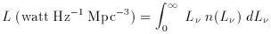
The luminosity
function is a distribution function, specifically the distribution of
luminosities of objects in a sample. Luminosity itself is difficult to
measure, since the total or bolometric luminosity requires both
accurate distance measurements and integration of each object's
spectrum over all frequencies. Generally we measure specific
luminosity, L , over a
given band, or range of frequency, so the units
of L are erg
sec-1 Hz-1. Then the luminosity function is
n(L), where
n(L) dL is the number of galaxies with
luminosity in the range L to
L + dL; n(L) has units Mpc-3 (watt
Hz-1)-1. The integral of n(L)
dL over all luminosities
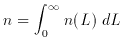
is just the density of galaxies, n.
, over a
given band, or range of frequency, so the units
of L are erg
sec-1 Hz-1. Then the luminosity function is
n(L), where
n(L) dL is the number of galaxies with
luminosity in the range L to
L + dL; n(L) has units Mpc-3 (watt
Hz-1)-1. The integral of n(L)
dL over all luminosities
is just the density of galaxies, n.
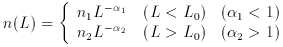
Note that if n(L) is
described by a power law, for L to be finite
requires that the power law index be less than -1 at high
luminosities, and greater than -1 at low luminosities, where L is the
total luminosity of all galaxies in a unit volume, i.e.,
A simple combination of power laws is often a useful approximate form to
assume for a luminosity function, i.e.,
What we know about luminosity functions generally comes from the
distribution of fluxes in a survey which is complete in some way. The
best is a volume-limited sample (meaning every galaxy in the volume
has been measured). This is rarely available, since all surveys have
some minimum detectable flux, Smin, which translates into a cutoff
distance rcut = sqrt(L / 4
is independent of position. In general n is a strong function of
position; it varies by several orders of magnitude between rich
clusters and voids; indeed, the study of this function is the main
subject of this course.
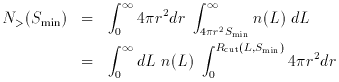
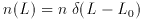
If the distribution of objects is homogeneous, so that n is a
constant independent of position, which presumably olds when we
average over very large scales, then we can easily evaluate some
simple integrals of the luminosity function which apply to a flux
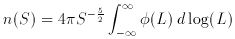
limited sample. The number of objects brighter than the minimum flux
Smin is just given by
where we have simply interchanged the integration over volume and over
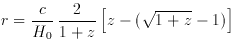
luminosity. (Note: the distance r, which on small scales is simply
cz / H0, generalizes in a Friedman universe with
see Condon (1984a).
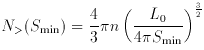
In the simplest case of ``standard candles'' the
luminosity function is
so that
In magnitude notation N>(Smin)
In a flux limited sample the contribution to n(s) of sources of
different luminosities is most easily seen in
von Hoerner's (1973)
``visibility function'':
whose dimensions are watt3/2 Hz-3/2
pc-3, which is usually converted to
Jy3/2. A plot of log
(see Condon 1984a,
b).
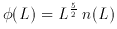
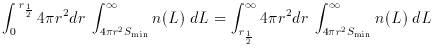
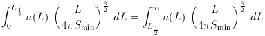
A useful integral of the luminosity function gives the median
distance to objects in a flux limited sample, r1/2, given by
where again we can interchange integration to get
where L1/2 = 4
where x = log L1/2, which is the obvious median value of
 Smin) which is a function of luminosity. So the sample
size is a function of luminosity. This bias can be corrected if we
know that the distribution of galaxies is homogeneous, i.e., that the
total density
Smin) which is a function of luminosity. So the sample
size is a function of luminosity. This bias can be corrected if we
know that the distribution of galaxies is homogeneous, i.e., that the
total density
 = 0,
= 0,  = 1 to
 Smin-3/2
becomes N<(m)
m0.6. The
``differential source count`` function, n(Smin) =
-dN> (Smin) / dSmin depends
on Smin to the minus 5/2 power, and the total flux from all
sources is
proportional to
Smin-3/2
becomes N<(m)
m0.6. The
``differential source count`` function, n(Smin) =
-dN> (Smin) / dSmin depends
on Smin to the minus 5/2 power, and the total flux from all
sources is
proportional to  S
n(S) dS which diverges. This is a statement of
Olber's paradox, which can only be resolved in a Euclidian universe if
the luminosity function evolves, i.e., changes with time. The only
tracers for which we have complete flux limited samples reaching to
large redshifts (z > 1) are QSO's and radio sources, both of which
apparently have luminosity functions which evolve strongly on
cosmological time scales.
S
n(S) dS which diverges. This is a statement of
Olber's paradox, which can only be resolved in a Euclidian universe if
the luminosity function evolves, i.e., changes with time. The only
tracers for which we have complete flux limited samples reaching to
large redshifts (z > 1) are QSO's and radio sources, both of which
apparently have luminosity functions which evolve strongly on
cosmological time scales.
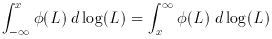
 (L) vs. log L immediately shows what range of
luminosities contribute most to a flux limited sample, since
(L) vs. log L immediately shows what range of
luminosities contribute most to a flux limited sample, since
 Smin r1/22. This can easily be
evaluated for n(L) having the
simple form of equation 1. For example, if n2 = 0 and
Smin r1/22. This can easily be
evaluated for n(L) having the
simple form of equation 1. For example, if n2 = 0 and  1 = 0 [i.e., a
step function n(L)], we find simply that r1/2 is 0.64
sqrt(L0 / 4
Smin). Using
(L) equation 6 becomes simply
1 = 0 [i.e., a
step function n(L)], we find simply that r1/2 is 0.64
sqrt(L0 / 4
Smin). Using
(L) equation 6 becomes simply
 (L) when plotted vs. log L.