


In Figure 1 I show the distribution of galaxies
of various
luminosity in a volume-limited sample through the Virgo, Coma and
Hercules superclusters. We use supergalactic
coordinates Y and Z
in km/s, respectively, in a sheet
0  X < 10
h-1 Mpc. Bright
galaxies (MB -
20.3) are plotted as red dots, galaxies
-20.3 < MB -
19.7 as black dots, galaxies
-19.7 < MB - 18.8 as
open blue circles, galaxies
-18.8 < MB -
18.0 as green circles
(absolute magnitudes correspond to Hubble parameter h = 1).
High-density regions are the Local, the Coma and the Hercules superclusters in the lower left, lower
right and upper right corners,
respectively. The long chain of galaxies between Coma and Hercules superclusters is called the Great
Wall. Actually it is a filament.
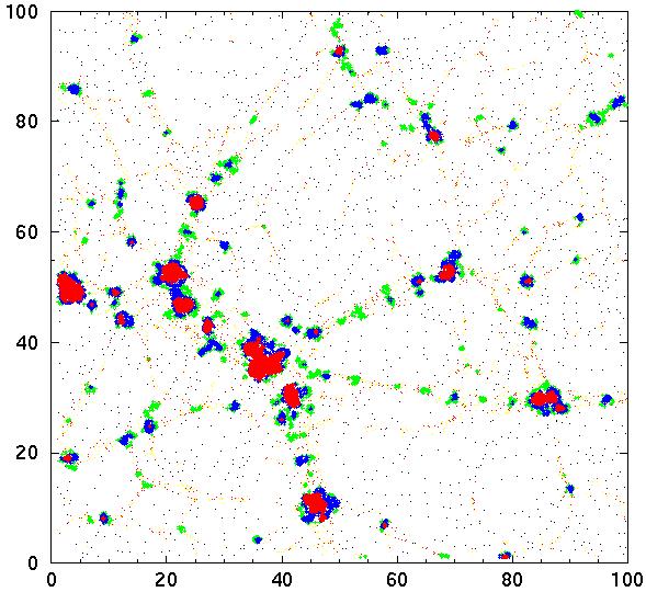
For comparison, the distribution of particles in a 2-dimensional
simulation is also plotted in a box of side-length 100
h-1 Mpc.
Different colors indicate the density value of the particle
environment. Particles in voids (density
X < 10
h-1 Mpc. Bright
galaxies (MB -
20.3) are plotted as red dots, galaxies
-20.3 < MB -
19.7 as black dots, galaxies
-19.7 < MB - 18.8 as
open blue circles, galaxies
-18.8 < MB -
18.0 as green circles
(absolute magnitudes correspond to Hubble parameter h = 1).
High-density regions are the Local, the Coma and the Hercules superclusters in the lower left, lower
right and upper right corners,
respectively. The long chain of galaxies between Coma and Hercules superclusters is called the Great
Wall. Actually it is a filament.
For comparison, the distribution of particles in a 2-dimensional
simulation is also plotted in a box of side-length 100
h-1 Mpc.
Different colors indicate the density value of the particle
environment. Particles in voids (density
 < 1) are shown as
black dots; particles in the density interval
1
< 5
form filaments of galaxies (orange dots); particles with densities
5
< 10 (green dots)
form groups of galaxies; particles
with 10
< 20 (blue dots)
form clusters; and particles
with
< 1) are shown as
black dots; particles in the density interval
1
< 5
form filaments of galaxies (orange dots); particles with densities
5
< 10 (green dots)
form groups of galaxies; particles
with 10
< 20 (blue dots)
form clusters; and particles
with
 20 (red dots) are in very rich clusters.
Densities are expressed in units of the mean density in the
simulation; they are calculated using a smoothing length of
1 h-1 Mpc. Three-dimensional simulations have similar
behaviour. This
Figure emphasizes that particles in high-density regions simulate
matter associated with galaxies, and that the density of the particle
environment defines the type of the structure. In both Figures we see
the concentration of galaxies or particles to clusters and filaments,
and the presence of large under-dense regions. There exists, however,
one striking difference between the distribution of galaxies and
simulated particles - there is a population of smoothly distributed
particles in low-density regions in simulations, whereas in the real
Universe voids are completely empty of any visible matter. This
difference is due to differences of the evolution of matter in under-
and over-dense regions.
20 (red dots) are in very rich clusters.
Densities are expressed in units of the mean density in the
simulation; they are calculated using a smoothing length of
1 h-1 Mpc. Three-dimensional simulations have similar
behaviour. This
Figure emphasizes that particles in high-density regions simulate
matter associated with galaxies, and that the density of the particle
environment defines the type of the structure. In both Figures we see
the concentration of galaxies or particles to clusters and filaments,
and the presence of large under-dense regions. There exists, however,
one striking difference between the distribution of galaxies and
simulated particles - there is a population of smoothly distributed
particles in low-density regions in simulations, whereas in the real
Universe voids are completely empty of any visible matter. This
difference is due to differences of the evolution of matter in under-
and over-dense regions.

| 
|
Figure 1. The distribution of galaxies (upper panel), and particles in a 2-D simulation (lower panel). For explanations see text | |
Zeldovich [60] and Einasto, Jõeveer & Saar [24] have shown that the density evolution of matter due to gravitational instability is different in over- and under-dense regions. The evolution follows approximately the law
| (1) |
where d0 is a parameter depending on the amplitude of
the density
fluctuations. In over-dense regions d0 > 0, and the
density
increases until the matter collapses and forms pancake or filamentary
systems [6]
at a time
t0; thus the formula can be applied
only for t
t0. In under-dense regions we have
d0 < 0 and the
density decreases, but never reaches zero (see
Figure 2).
In other words, there is always some dark matter in under-dense
regions. At the time when over-dense regions collapse the density in
under-dense regions is half of the original (mean) density. In order
to form a galaxy the density of matter in a given region must exceed a
certain critical value
[44],
thus galaxies cannot form in
under-dense regions. They form only after the matter has flown to
over-dense regions: filaments, sheets, or clusters; here the
formation occurs in situ.

| 
|
Figure 2. Left: Density evolution in over- and under-dense regions (solid and dashed lines, respectively) for two epochs of caustics formation. Right: Density perturbations of various wavelengths. Under-dense regions (D < 1) become voids; strongly over-dense regions (D > 1.3) - superclusters (cluster chains); moderately over-dense regions (1 < D < 1.3) - filaments of groups and galaxies. | |
Consider the distribution of matter as a superposition of several sinusoidal waves of amplitude ai and period pi around the mean density Dm
| (2) |
Gravitational instability determines the evolution of these density perturbations: large high over-dense regions become superclusters; weakly over-dense regions become small filaments of galaxies and groups; under-dense regions become voids, see Figure 2. The fine structure of superclusters is defined by perturbations of medium wavelength, the structure of clusters by small-scale perturbations.