4.2. Correlation function

The two-point correlation function (r) is defined as the excess over Poisson of the joint probability of finding objects in two volume elements separated by r and averaged over a very large volume [42]. We shall use the term ``correlation function'' for its estimate, determined in a limited volume, and calculate it using the formula:

(7)

where < DD(r) > is the number of pairs of galaxies (or clusters of galaxies) in the range of distances r±dr / 2, dr is the bin size, < RR(r) > is the respective number of pairs in a Poisson sample of points, n and n_R are the mean number densities of clusters in respective samples, and brackets < ... > denote the ensemble average. The summation is over the whole volume under study, and it is assumed that the galaxy and Poisson samples have identical shape, volume and selection function.

Both the correlation function and the power spectrum characterise the distribution of galaxies, clusters and superclusters. In an ideal case in the absence of errors, and if both functions are determined in the whole space, they form a mutual pair of Fourier transformations:

	(8)
	(9)

These formulae are useful when studying theoretical models or results of numerical simulations. For real samples they are of less use since observational errors and selection effects influence these functions in a different way. Also they reflect the spatial distribution of objects differently, thus they complement each other.

There exists a large body of studies of the correlation function of galaxies and clusters. Already early studies have shown that on small scales the correlation function can be expressed as a power law (see [42]):

(10)

where 1.8 is the power index, and r₀ 5 h^-1 Mpc is the correlation length. The correlation function of clusters of galaxies is similar, but shifted to larger scales, i.e. it has approximately the same power index but a larger correlation length, r₀ 25 h^-1 Mpc. On small scales the correlation function reflects the fractal dimension, D = 3 - , of the distribution of galaxies and clusters [54]. On large scales the correlation function depends on the distribution of systems of galaxies.

In order to understand better how different geometries of the distribution of galaxies and clusters are reflected in the properties of the correlation function and power spectrum, we shall construct several mock samples with known geometrical properties, and calculate both functions. Here we use results of the study of geometrical properties of the correlation function [25, 20].

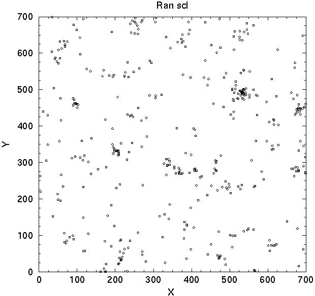
The correlation function is determined by mutual distances of galaxies (or clusters) in real space, thus this function depends directly on the structure of galaxy systems themselves (on small separations which are comparable to sizes of these systems), and on the distribution of galaxy systems (on separations which exceed the dimensions of galaxy systems). To see these effects separately we have constructed two series of mock samples. In the first series we change the distribution of galaxies on small scales following [25], in the second series we change the distribution of systems themselves [20]. In the first case we consider test particles as galaxies; they form two populations - clusters and field galaxies. Clusters are located randomly in a cube of size L = 100 h^-1 Mpc; clusters have a varying number of member galaxies from 12 to 200, and an abundance and mass distribution in accordance with the observed cluster mass distribution (see the next subsection). Inside clusters galaxies are located randomly with an isothermal density distribution. For the field population we consider three cases. In the first model there is no field population at all; in Figure 4 this model is designated gal248 (it contains 248 clusters). The second model has 200 clusters and 6000 randomly located field galaxies (designated as g2006t). The third model has also 200 clusters, but field galaxies are located in filaments - each filament crosses one cluster in either x, y, or z-axis direction, randomly chosen, and has 30 galaxies; this sample is designated as g20030. The total number of galaxies in clusters and in the field population in the two last models is approximately equal.

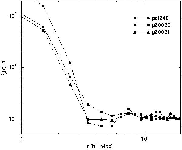
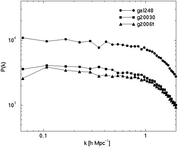
Figure 4. The distribution of galaxies and clusters in random mock models (upper left and right panels, respectively), respective correlation functions (middle panels) and power spectra (lower panels). For explanations see text.

The distribution of galaxies in a sheet of thickness 15 h^-1 Mpc of the model g20030 is shown in the upper left panel of Figure 4. In the other two models the distribution of clusters is similar, but field galaxies are distributed randomly or are absent. The correlation functions and power spectra of all three models are plotted in the middle and lower left panels, respectively. We see that the slope (power law index) of the correlation function at small separations is 3 in the pure cluster model, and 1.8 in other two models. These differences are due to the difference in the effective fractal dimension: D = 3 - 0 for the pure cluster model (clusters are spherically symmetrical); and D 1.2 in a mixture of spherically symmetrical clusters and one-dimensional filaments. The power index depends on the partition of galaxies between the clustered and the field populations. On scales of r 3 h^-1 Mpc the correlation function changes sharply. In the pure cluster model it has small negative values for r > 3 h^-1 Mpc, while in the random field models (r) 0 for r > 3 h^-1 Mpc. In the model with filaments the correlation function is positive but has a smaller power index, of 1.2. The change of the power index occurs on a scale equal to the diameter of clusters of galaxies. On larger scale the behaviour of the correlation function depends on properties of the field population and on the distribution of clusters. In the absence of the field there are only a few close neighbours of clusters, hence the slightly negative value of the correlation function; on larger scales the level of the correlation function reflects the distribution of clusters; clusters are distributed randomly and the level is approximately zero. In the random field model galaxies are located also in the vicinity of clusters and the zero level of the correlation function begins immediately beyond the end of cluster galaxies. In the filamentary model the effective power index of the correlation function reflects the mean fractal dimension of filaments.

The power spectrum of all three models has a similar shape. On small scales the power index is negative and depends on the clustering law of galaxies in clusters. On larger scales the shape of the power spectrum depends on the distribution of galaxies and clusters on respective scales. Because both clusters and field galaxies are essentially randomly distributed (the location of filaments is also random), the spectrum has a zero power index as expected for a random distribution. The amplitude of the power spectrum depends on the fraction of galaxies in clusters. In the pure cluster model the amplitude is much higher, and the difference in the amplitude depends on the fraction of galaxies in clusters. This effect is similar to the influence of the void population discussed above.

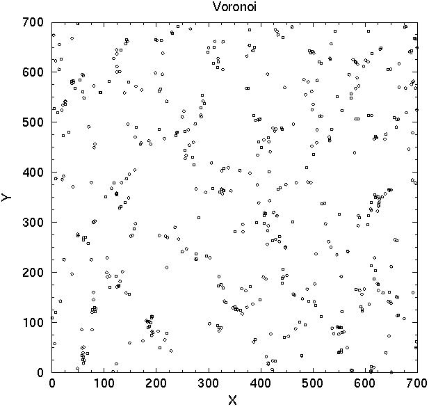
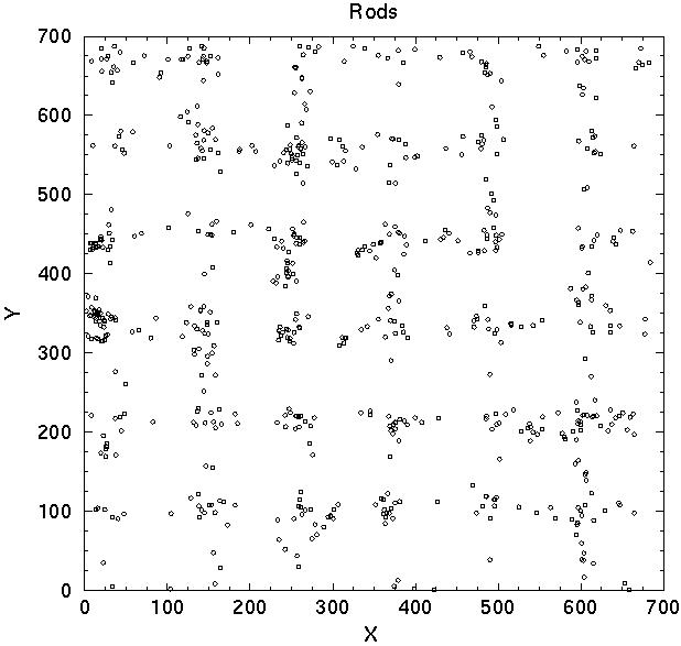
Now we shall discuss models of the cluster distribution. We do not include the population of galaxies; instead we shall investigate how different distribution of clusters affects the correlation function and power spectrum. Here we assume that a fraction of clusters are located in superclusters, the rest form a field cluster population. We consider again three models: randomly distributed superclusters, regularly spaced superclusters, and superclusters formed by the Voronoi tessellation model. In the Voronoi model centers of voids are located randomly, and clusters are placed as far from void centres as possible. These models differ in their degree of regularity of the distribution of superclusters. The random supercluster model has no regularity and no built-in scale. The Voronoi model has a characteristic scale - the mean diameter of voids (determined by the number of voids in the sample volume), but no regularity in the distribution of voids. In the regular model superclusters are located randomly along rods which form a regular rectangular grid of step size 120 h^-1 Mpc; this scale defines the mean size of voids between superclusters, and also puts voids to a semiregular honeycomb-like lattice. In addition a field population of isolated randomly located clusters is present in this model.

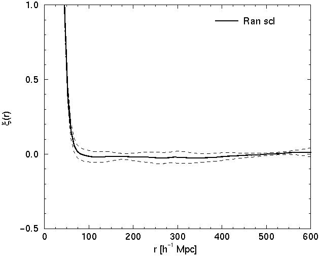
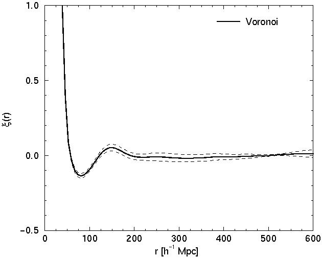
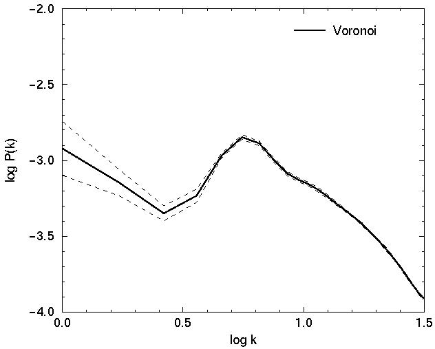
The distribution of clusters of the random, Voronoi, and regular model are shown in the upper panels of Figure 4 and 5; correlation functions are given in the middle panels, and power spectra in the lower panels. We see that on small scales all correlation functions are identical; power spectra on small wavenumbers are also identical. This is due to the fact that on these scales both functions are determined by the distribution of clusters within superclusters; and superclusters in all models were generated using the same algorithm as in generating galaxies in clusters. On larger scales there are important differences between models. In the random supercluster model the correlation function approaches zero at r > 80 h^-1 Mpc. In the Voronoi model it has a minimum around r 80 h^-1 Mpc, followed by a secondary maximum at r 150 h^-1 Mpc; thereafter it approaches zero. The correlation function of the regular rod model is oscillating: it has a series of regularly spaced maxima and minima with a period of ~ 120 h^-1 Mpc; the amplitude of oscillations decreases with increasing separation. The power spectrum of the random supercluster model is flat and featureless on large scales, while in the Voronoi and regular models it has a sharp maximum at wavenumber, which corresponds to the mean diameter of voids in models and to the period of oscillations of the correlation function. The shape of the power spectrum on large scales of these two models is, however, different.

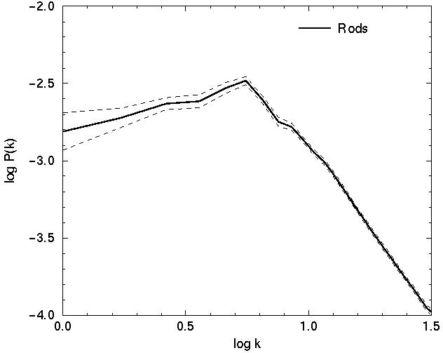
Figure 5. The distribution of clusters in Voronoi and regular mock models (upper left and right panels, respectively), respective correlation functions (middle panels) and power spectra (lower panels). For explanations see text.

These mock samples illustrate properties of the correlation function and power spectrum on small and large scales and their dependence on the distribution of galaxies and clusters within systems and on the distribution of systems themselves. The correlation function of clusters of galaxies in rich superclusters is shown in the right panel of Figure 3. This function is oscillating with a period which corresponds to the maximum of the power spectrum at k = 0.05 h Mpc^-1, seen in the left panel of the same Figure. We note that a periodicity of the distribution of high-density regions with the same period has been observed in the direction of the galactic poles by Broadhurst [8]. All these facts suggests that there exists a preferred scale of ~ 130 h^-1 Mpc in the Universe, and possibly also some regularity in the distribution of the supercluster-void network.